Radhika Chenniappan*![]() | Chandrasekaran Viswanathan
| Chandrasekaran Viswanathan![]() | Vijay Anand Duraisamy
| Vijay Anand Duraisamy![]() |
|
© 2025 The authors. This article is published by IIETA and is licensed under the CC BY 4.0 license (http://creativecommons.org/licenses/by/4.0/).
OPEN ACCESS
The detection of focal Electroencephalogram (EEG) signal in the human brain is important to detect and diagnose Epilepsy disease. In this work, the EEG signals can be differentiated into Focal Signal (FS) and Non-Focal Signal (NFS) for Epileptic Seizure detection in the human brain. This proposed system has been designed with preprocessing, signal decomposition module, intrinsic features computations and its optimization with classification and severity diagnosis module. The Chebyshev filter is used in preprocessing stage which suppresses the noise components in the acquired EEG signals and the preprocessed signals are decomposed using Weighted Empirical Mode Decomposition (WEMD). The textural intrinsic features have been computed from the decomposed Intrinsic Mode Function (IMF) sub bands and they are classified by the proposed EEGNet classification architecture, which classifies the test EEG signal into either FS or NFS. Then, FS can be diagnosed into three severity level cases as mild, moderate and severe using the EEGNet architecture. This proposed system has been tested with two independent EEG datasets in order to analyze the stability and robustness of the EEG classification process.
EEG, focal, features, classifications, Epilepsy
The diseases in the human brain can be detected using either imaging modality techniques such as Computer Tomography (CT) or Magnetic Resonance Imaging (MRI) or signaling modality techniques [1-3]. The earlier techniques are mostly used for detecting the tumors or Alzheimer diseases which are relating to brain region. The later technique is used for detecting the Epilepsy disease which is relating to human brain and it is identified as one of the neurological disorders. The EEG electrodes are placed over the human brain and the EEG signals are captured through these electrodes from various regions of the human brain. The cells in the human brain are damaged which produces the FS from the epileptic region of the brain. The NFS are captured from the non-epileptic region of the brain [4-7]. Both EEG signals are analog in nature and the Epileptic disease can be detected by analysing these FS and NFS. The World Health Organization (WHO) report 2023 states that approximately 70 million of humans are affected by this Epilepsy disease around the world. The EEG capturing module captured the long-term EEG signals or recordings from the patients and these long-term EEG recordings have been analyzed by the experts or neurologist to locate the occurrence of these abnormal spikes in the brain region. The Epilepsy detection through the neurologist consumed more time, which is not appropriate for identifying this disease for the larger population groups or countries [8, 9].
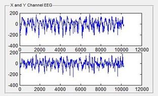
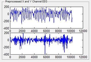
Hence, the automatic detection of the epilepsy through FS detection process has been done by the Artificial Intelligence (AI) techniques. These AI techniques extract the features directly from the time series, frequency series or time-frequency series EEG signals which are captured by the various channels of the electrodes. These features are fed into either machine learning algorithm or deep learning algorithm to detect FS from the NFS. The machine learning algorithms such as Support Vector Machine (SVM), Random Forest (RF), Decision trees, K-Nearest Neighbour (KNN) used frequency series for identifying the FS for Epileptic seizure detection. The non-linear properties of the frequency series affect the classification rate of the machine learning algorithms [10]. Hence, deep learning algorithm has been developed and used by many researchers from the past decade for the automatic classification of FS over NFS. The frequently used deep learning algorithms are LeNet, AlexNet, GoogleNet, Inception and Visual Geometry Group (VGG). These deep learning algorithms are mostly used time series or time-frequency series signals for obtaining the higher EEG signal classification rate. This research work proposes a novel EEGNet deep learning architecture for classifying FS and NFS for epileptic seizure detection. Figure 1(a) is FS representation and Figure 1(b) is NFS representation.
In present research studies, there are numerous FS and NFS automatic detection methods and these works are mainly focuses to perform the automatic classification process. However, these works have certain limitations: not involved any critical clinical diagnosis process and higher algorithm design complexity. Therefore, the proposed aim of this research work is to develop novel fully automated methods for FS and NFS signal classifications.
Figure 1. (a) EEG-FS (b) EEG-NFS
By utilising an advanced deep learning and cutting-edge technologies for early seizure prediction and individual treatment planning, the suggested approaches proposed in this research work seek to solve unmet clinical needs in the management of Epilepsy. This entails recognising preictal patterns in EEG signals to offer prompt intervention warnings and modifying treatment plans in accordance with the traits and reactions of each unique patient. By providing more precise and individualised solutions for managing Epilepsy, these strategies fill unmet clinical needs and open the door to better patient outcomes.
The contributions of this proposed research work are highlighted in the following points.
The contents of this research paper have been organized into various sections. In section 2, various FS and NFS detection conventional methods are analyzed with their limitations. The proposed EEG signal classification method has been stated in section 3 and the results are analyzed and discussed in section 4. In section 5, conclusion is finally depicted.
This section states the literature survey of the traditional works which are related to the EEG signal classification process using various focused machine learning and artificial intelligence techniques. Moreover, this section investigates the advantages and limitations of each traditional methods for framing the problem related with EEG signal classifications.
Abenn et al. [11] used band pass filter to filter the noise frequency components in the EEG signals. Then, the non-linear classification architecture such as Light Gradient Boosting Machine (LGBM) based on the Gradient boosting algorithm has been used in this work to perform the classification of the EEG signal into either FS or NFS. The authors obtained 96.5% SDSe, 96.1% SDSp, 96.3% SP, 95.7%SA and 95.1% FS on BEBA database and also attained 96.5% SDSe, 96.3% SDSp, 95.8% SP, 95.6%SA and 96.3% FS on CHB-MIT database. Ahmad et al. [12] used Butterworth filter to suppress the noise components from the obtained EEG signals through various electrode channels. Then, DWT was applied on these filtered signals to obtain the decomposed coefficients at various stages. Then, Fractal Dimension-based Non-Linear (FDNL) transformation method was involved in this work to obtain the decomposition coefficients and these FDNL coefficients were classified by the proposed Bagged Tree Based Classifier (BTBC). The authors obtained 97.1% SDSe, 97.3% SDSp, 97.1% SP, 96.4%SA and 96.9% FS on BEBA database and also attained 97.1% SDSe, 97.1% SDSp, 96.8% SP, 96.2%SA and 97.1% FS on CHB-MIT database.
Kantipudi et al. [13] performed the EEG signal classification using the feature enhanced classification algorithm. This method used Finite Linear Haar wavelet-based Filtering (FLHF) approach for detecting and removing the noise contents from the signal and then Fractal Dimension (FD) decomposition method has been used to decompose the filtered signals into various number of lower and higher sub bands. The coefficients in these sub bands were optimized using the proposed Grasshopper Bio-Inspired Swarm Optimization (GBSO) method which optimized the fine-tuned features from the signal components. These optimized fine-tuned components were further classified by the Temporal Activation Expansive Neural Network (TAENN) classification algorithm. The authors obtained 97.2% SDSe, 97.9% SDSp, 97.4% SP, 97.0%SA and 97.4% FS on BEBA database and also attained 97.8% SDSe, 97.2% SDSp, 97.1% SP, 97.4%SA and 97.5% FS on CHB-MIT database.
Mathe et al. [14] used two different types of classification algorithms as Customized Deep Network (CDN) and the Support Vector Machine (SVM) classifier. The CDN classifier has been used for detecting and removing the artifact components from the source EEG signal. The artifact removed EEG signals were classified further through the SVM classification algorithm which classified the signal into either FS or NFS. For this classification process by SVM, the intrinsic mode decomposition was used and applied on the artifact removed signals for extracting the intrinsic features. The authors obtained 96.9% SDSe, 96.5% SDSp, 96.9% SP, 96.1%SA and 95.3% FS on BEBA database and also attained 96.8% SDSe, 96.8% SDSp, 96.3% SP, 96.0%SA and 96.9% FS on CHB-MIT database.
Akbari et al. [15] decomposed the EEG signal using Empirical Wavelet Transform (EWT) which produced both lower order and higher order decomposition filter coefficients. This EWT exhibited the properties of Discrete Wavelet Transform (DWT) for obtaining lower component losses during the signal decomposition. The authors obtained 95.3% SDSe, 94.8% SDSp, 95.1% SP, 94.7%SA and 94.9% FS on BEBA database and also attained 96.1% SDSe, 95.2% SDSp, 95.2% SP, 95.2%SA and 95.9% FS on BEBA database. Hussain et al. [16] used Long Short-Term Memory Neural Networks (LSTMNN) method for detecting the epileptic seizure. The memory module of the existing system has been modified using dynamic mode of memory elements which were used for extracting the fine-tuned features from the source signals. These fine-tuned features were fed into the LSTMNN classifier for performing the classification of EEG signals. The authors obtained 93.9% SDSe, 93.7% SDSp, 94.2% SP, 93.2%SA and 94.8% FS on BEBA database [17] and also attained 95.3% SDSe, 94.8% SDSp, 94.9% SP, 94.8%SA and 94.7% FS on CHB-MIT database [18].
Mahsa Zeynali et al. [19] used transformer-based model for signal decomposition in a focal and non-focal signal classification system. This transformer-based decomposition model used the Power Spectral Density (PSD) approach for obtaining the decomposition coefficients with respect to the frequency domain patterns in this work. This method further uses a binary deep learning algorithm to differentiate the decomposed frequency domain patterns for EEG signal classification process. Si et al. [20] used a transformer decomposition algorithm-based ensemble deep learning model for the EEG signals classifications. This transformer decomposition algorithm produced frequency domain features and these features were classified using an ensemble deep learning algorithm. The authors obtained 95% average classification accuracy using this transformer decomposition algorithm in this work.
Mathe et al. [14] used two different types of classification algorithms as Customized Deep Network (CDN) and the Support Vector Machine (SVM) classifier. The CDN classifier has been used for detecting and removing the artifact components from the source EEG signal. The artifact removed EEG signals were classified further through the SVM classification algorithm which classified the signal into either FS or NFS. For this classification process by SVM, the intrinsic mode decomposition was used and applied on the artifact removed signals for extracting the intrinsic features. The authors obtained 96.9% SDSe, 96.5% SDSp, 96.9% SP, 96.1%SA and 95.3% FS on BEBA database and also attained 96.8% SDSe, 96.8% SDSp, 96.3% SP, 96.0%SA and 96.9% FS on CHB-MIT database. Abenn et al. [11] used band pass filter to filter the noise frequency components in the EEG signals. Then, the non-linear classification architecture such as Light Gradient Boosting Machine (LGBM) based on the Gradient boosting algorithm has been used in this work to perform the classification of the EEG signal into either FS or NFS. The authors obtained 96.5% SDSe, 96.1% SDSp, 96.3% SP, 95.7%SA and 95.1% FS on BEBA database and also attained 96.5% SDSe, 96.3% SDSp, 95.8% SP, 95.6%SA and 96.3% FS on CHB-MIT database.
Akbari et al. [15] decomposed the EEG signal using Empirical Wavelet Transform (EWT) which produced both lower order and higher order decomposition filter coefficients. This EWT exhibited the properties of Discrete Wavelet Transform (DWT) for obtaining lower component losses during the signal decomposition. The authors obtained 95.3% SDSe, 94.8% SDSp, 95.1% SP, 94.7%SA and 94.9% FS on BEBA database and also attained 96.1% SDSe, 95.2% SDSp, 95.2% SP, 95.2%SA and 95.9% FS on BEBA database. Hussain et al. [16] used LSTMNN method for detecting the epileptic seizure. The memory module of the existing system has been modified using dynamic mode of memory elements which were used for extracting the fine-tuned features from the source signals. These fine-tuned features were fed into the LSTMNN classifier for performing the classification of EEG signals. The authors obtained 93.9% SDSe, 93.7% SDSp, 94.2% SP, 93.2% SA and 94.8% FS on BEBA database and also attained 95.3% SDSe, 94.8% SDSp, 94.9% SP, 94.8%SA and 94.7% FS on CHB-MIT database.
In accordance with the existing studies in literature survey section, it is observed that most of the methods used artificial intelligence techniques to obtain the higher positive signal classification rate with a minimum number of input signal patterns. If the traditional system is tested with a higher number of EEG signals, the classification rate is reduced. Therefore, the limitations of these traditional signal classification process have been overcome by developing a novel EEG signal classification system in this work.
In this work, the EEG signals can be differentiated into FS and NFS for Epileptic Seizure detection in the human brain. This proposed system has been designed with preprocessing, signal decomposition module, intrinsic features computations and its optimization with classification and severity diagnosis module. The Chebyshev filter is used in preprocessing stage which suppresses the noise components in the acquired EEG signals and the preprocessed signals are decomposed using WEMD. The textural intrinsic features have been computed from the decomposed IMF sub bands and they are classified by the proposed EEGNet classification architecture, which classifies the test EEG signal into either FS or NFS. Then, FS can be diagnosed into three severity level cases as mild, moderate and severe using the EEGNet architecture.
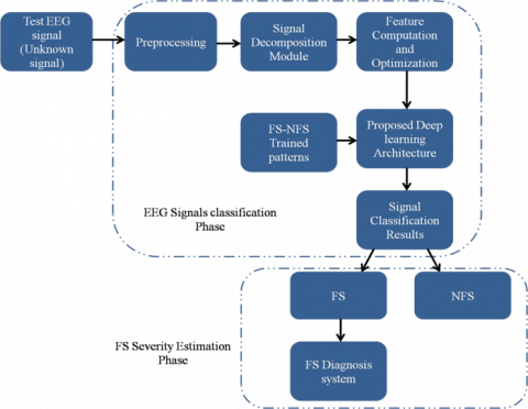
Figure 2. (a) FS and NFS classification system in learning stage (b) EEG signal classification and FS severity estimation systems in testing stage
Figure 2(a) is the FS and NFS classification system in learning stage and Figure 2(b) is the EEG signal classification and FS severity estimation systems in testing stage.
(1) Preprocessing with Scaled Chebyshev Filter (SCF)
The EEG signals which are captured by the set of electrodes with respect to various channels are affected by the noise components. The noise contents and its variations in the acquired EEG signals create the greater impact in achieving the higher signal classification rate. Hence, it is important to suppress the noise contents in the acquired EEG signals before it has been processed by the classification module of the proposed EEG signal classification system.
For noise suppression process in signal, Finite Impulse Response (FIR) and Infinite Impulse Response (IIR) filters have been used by many researchers from the past decades. The IIR filter has faster responses than the FIR filtering process for signals. The recursive behaviour of the IIR system has been designed with a feedback system where the present output of the filtering system has been depending on the past input and output of the filtering system. This filter has been used to select one band frequency of the signal from the set of band frequencies. The functional speed of the Chebyshev filter is more than the Butterworth filter and other signal processing filters due to their recursion mode process during filtering of signals where the other mode process during filtering of signals whereas the other signal filters used a convolution mode process for filtering. Moreover, the functional transition between pass to stop bands is relatively higher in Chebyshev filter than in the other signal processing filters. This sharper transition process between the stop and pass bands can be achieved even in lower orders which produces small frequency synthesis errors. The odd and even degrees have been used for designing the Chebyshev filter with polynomial curve. The maximum power is required for odd degree-based Chebyshev filter. This drawback can be resolved by using even even-degree-based based Chebyshev filter for filtering the signals. Hence, this work uses SCF for filtering both FS and NFS.
The polynomial of even degree based SCF is depicted in the following equation.
$p_n(\omega)=\cos (n * \arccos (\omega))$ (1)
The frequency of the SCF has been deployed in this following equation.
$\omega=\sqrt{\omega^2\left(1-p^2\right)+p^2}$ (2)
where, $p$ is SCF polynomial root factor and it is determined with the order of the SCF which is given in the following equation.
$p= \pm \cos \left(\frac{n-1}{2 n} \pi\right)$ (3)
This SCF has been applied on both FS and NFS in order to suppress the noise contents in the acquired EEG signals.
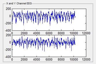
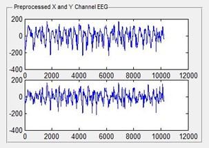
Figure 3. (a) FS before applying SCF (b) FS after applying SCF (c) NFS before applying SCF (d) NFS after applying SCF
Figure 3(a) and Figure 3(b) are the illustrations of FS before and after applying the SCF, Figure 3(c) and Figure 3(d) are the illustrations of NFS before and after applying the SCF.
(2) WEMD algorithm
It is a technique which is used to decompose the non-stationary signals for computing the fine-tuned intrinsic set of features. The decomposition process produces a number of intrinsic modes at various stages of the decomposition. This method uses multi-resolution process to obtain the intrinsic modes from the non-linear and non-stationary signals. It produces the intrinsic modes which are based on the different resolutions. The conventional multi resolution process such as Discrete Wavelet Decomposition (DWD), Contourlet Decomposition (CD) decomposes the signal and produces the intrinsic modes with the same resolution. Hence, the same set of intrinsic features has been extracted from their intrinsic modes which cannot be used for classifying the signal into various types, in order to eliminate such issues in conventional multi resolution process.
Most of the researchers used traditional Empirical Mode Decomposition (EMD) and Empirical Wavelet Transform (EWT) methods to decompose the EEG signals for classification process. During the decomposition of the signal into intrinsic modes and residual modes through the traditional EMD method, the errors of the residual modes in the decomposed coefficients are high and also it exhibits the minimum differences between the decomposed intrinsic modes. Hence, the signal differentiation rate through the EMD and EWT are low which is identified as the main limitation of this traditional decomposition models. This limitation has been overcome by proposing the WEMD method which is the modification of the traditional EMD method through the weighting modes. The weighted index is computed from the EEG signals through the local maxima and local minima and this weighted index is used to reduce the residual mode errors and exhibits the significant differences between the decomposed intrinsic modes. This increases the signal detection accuracy, which is the main advantage of this proposed WEMD.
The WEMD has been used in this work to produce different and variational intrinsic sub bands which are based on different resolution for the computation of the variational intrinsic features.
The WEMD algorithm for signal decomposition uses sifting function which is used to produce the number of intrinsic modes. The WEMD produces IMF and residual components. The IMF represents the decomposed coefficients of the time series signal and the residual component represents the trend of the EEG signal.
The WEMD algorithm for EEG signal decomposition process can be explained through the following steps.
Step 1:
Find the local maxima $\left(L_{m a}\right)$ and the local minima $\left(L_{m i}\right)$ of the EEG signal and the EEG signal is represented by the following equation:
$x(t)=\sum_{j=1}^L h_i(t)+r(t)$ (4)
whereas, $x(t)$ is the EEG signal, $h_i(t)$ is the decomposed IMF and $r(t)$ is the residual band.
Step 2:
Compute weighted local maxima and weighted local minima of the EEG signal using the number of samples in upper envelope and lower envelope.
$W L_{m a}=N 1 * L_{m a}$ (5)
$W L_{m i}=N 2 * L_{m i}$ (6)
Step 3:
Compute Weighted local index $\left(W L_i\right)$ from the obtained weighted local maxima and local minima using the following equations.
$W L_i=\frac{W L_{m a} * W L_{m i}}{N 1+N 2}$ (7)
Step 4:
Find the weighted threshold between the weighted local maxima and weighted local minima using the following equation.
$W t_1=\frac{W L_{m a}+W L_{m i}}{2} * W L_i$ (8)
|
Pseudocode for IPF optimization by GA |
|
Input: IPF by N*N matrix; Output: Optimized IPF;
(a). Load IPF elements in first chromosome; (b). Load IPF elements in second chromosome; 5. Call single point crossover and mutation functions. Invoke crossover (chromosome1, chromosome2); If (crossover) is done Invoke mutation (chromosome1, chromosome2); If (mutation) is done Compute fitness function; Else Repeat step 5; Endif Endif
Compute E1=Minimum (Euclidean distances)
Compute E2=Minimum (Euclidean distances)
If (E==E1) Select patterns in chromosome1 and discard patterns in chromosome2; Else Select patterns in chromosome2 and discard patterns in chromosome2;
|
Step 5:
The IMF bands can be now separated from the EEG signal using the weighted threshold using the following equation:
$I M F 1=x(t)-W t_1$ (9)
After obtaining IMF1, step 1 to step 4 are repeated in order to get the new weighted threshold $\left(W t_2\right)$ at stage 2 as depicted by:
$I M F 2=I M F 1-W t_2$ (10)
Similarly, the remaining IMF bands can be obtained using the following equations.
$I M F 3=I M F 2-W t_3$ (11)
$I M F 4=I M F 3-W t_4$ (12)
$I M F 5=I M F 4-W t_5$ (13)
$I M F 6=I M F 5-W t_6$ (14)
After computing IMF6 band, there are no local maxima and local minima for computing the weighted threshold. Hence, the iteration has been stopped at this decomposition stage.
(3) Computation of IPF and its optimization
All the coefficients in six IMF bands are now formatted in two-dimensional matrix (IMF feature matrix) which is further used for computing the IPF. In this article, Skewness, Kurtosis, Energy and Entropy features have been computed from the IMF feature matrix for the differentiation of FS from NFS.
Skewness and Kurtosis
These features illustrate the shape behaviour of the signals. Hence, FS can be differentiated from the NFS through these textural features. The asymmetry distribution of the amplitude coefficients is represented by Skewness (third order texture feature) and the flat distribution of the amplitude coefficients are represented by Kurtosis (fourth order texture feature). The computational values of these texture features may vary from negative to positive index as illustrated by the following equations.
Skewness s $(x)=E\left[\left(\frac{x-E(x)}{\sqrt{\text { var }(x)}}\right)^3\right]$ (15)
where, $x$ is the two-dimensional feature matrix which has N rows and N columns respectively.
E(x) and var(x) are the mean and variance of the feature matrix and they have been computed using the following equations.
whereas,
$E(x)=\frac{1}{N} \sum_{i=1}^N x_i$ (16)
$\operatorname{Var}(x)=\frac{1}{N-1} \sum_{i=1}^N\left(x_i-E(x)\right)^2$ (17)
Kurtosis $K(x)=E\left[\left(\frac{x-E(x)}{\sqrt{\operatorname{var}(x)}}\right)^4\right]$ (18)
Entropy and Energy
The disorder of the EEG signal can be found by measuring the entropy and energy of the signal. The disorder of the signal is direct proportional to the energy and entropy of the signal and they are depicted in the following equations.
Entropy $H(x)=-\sum_x p(x) * \log (p(x))$ (19)
$\operatorname{Energy} E(x)=\sum_{t=-\infty}^{\infty} x(t)^2$ (20)
Table 1 is the illustration of computed IPF on both FS and NFS and it clearly shows that there are significant textural pattern differences between FS and NFS. These variation of the IPF are used by the classifier to classify whether the given test EEG signal is belonging to FS or NFS.
Table 1. Illustration of computed IPF on both FS and NFS
|
IPF |
EEG Signal Type |
|
|
FS |
NFS |
|
|
Skewness |
-0.60 |
-1.67 |
|
Kurtosis |
6.17 |
12.25 |
|
Entropy |
7.6*103 |
9.56*103 |
|
Energy |
8.0*104 |
1.3*105 |
The IPF have been computed for all the FS and NFS available in training dataset and hence the size of the computed IPF is high, which cannot be directly feed into the classifier for further classification process. Hence, they have to be optimized before it is fed into the classifier. Though there are numerous optimization algorithm available for features optimization, GA have been used in this work to optimize the computed IPF features. This IPF optimization process through GA has been explained in the following Algorithm.
(4) Classification
The classification module in the proposed EEG signal detection system is important which performs the classification of the input optimized features into either FS or NFS. In past decades, the EEG signals were differentiated by many researchers using machine learning algorithms such as Support Vector Machine (SVM) and Decision trees. These machine learning algorithms exhibits certain limitations that they require a larger number of EEG signals in both FS and NFS case which consumed more time period for the classification process. Hence, the deep learning algorithms has been developed and used by the researchers in the EEG signal classification process. There is numerous conventional deep learning algorithms are available for EEG signal classification process such as LeNet, AlexNet and Inception networks. These are non-customizable architectures where the internal layering modules are not able to modify. This brings this research work to propose the novel EEGNet architecture which is the extension of the conventional deep learning architecture.
The classification module of the EEGNet architecture can be operated in both training and testing phases. During training phase of the classification module, the optimized features are individually computed from FS and NFS and they are fed into the classifier in order to produce the individual training patterns for both FS and NFS. During testing phase of the classification module, the optimized features from the test EEG signal are fed into the classifier along with the individual training patterns which are obtained through the training phase of the classifier.
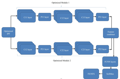
In this work, EEGNet deep learning architecture is proposed for the classification of the optimized features from the test EEG signal. The proposed EEGNet architecture for the feature classification process has been illustrated in Figure 4. This EEGNet architecture has been designed with Optimized Module1 (OM1) and Optimized Module2 (OM2). This proposed EEGNet architecture has been derived from the conventional AlexNet deep learning architecture where the number of internal layers has been enhanced in order to produce a greater number of significant set of features. The number of significant internal features decides the classification rate performance, where the number of significant internal features is directly proportional to the classification rate performance. The conventional AlexNet architecture was designed with 5 Convolutional layers and 3 pooling layers with Fully Connected Neural Networks (FCNN). The number of Convolutional layers in the conventional AlexNet has been improved by including a greater number of Convolutional layers. Moreover, the conventional AlexNet architecture functions as serial mode where the response of each internal layer is depending on the previous layer and hence it consumes more time period for the production of the internal features. This limitation has been resolved in the proposed EEGNet architecture by designing the internal layers as parallel structuring method which produce a greater number of significant features with less computational time period.
The IM1 constitutes with 3 Convolutional layers along with two pooling layers as described by the following equations.
$I M 1=\left\{\begin{array}{c} {Convolutional\ layers:}\ C 11\ {layer } \\ { C12\ layer\ and\ } C 13\ { layer } \\ { Pooling\ layers:}\ P 11\ { layer } \\ { and }\ P 12\ { layer }\end{array}\right.$ (21)
C11 layer: 128 filters with $5 * 5$ filter size
C12-layer: 256 filters with $7 * 7$ filter size
C13 layer: 512 filters with $9 * 9$ filter size
The IM2 constitutes with 3 Convolutional layers along with two pooling layers as described by the following equations.
$I M 2=\left\{\begin{array}{c}{ Convolutional\ layers: }\ C 21\ { layer }, \\ C 22\ { layer\ and }\ C 23\ { layer } \\ { Pooling\ layers: }\ P 21 \\ \text { layer and } P 22 \text { layer }\end{array}\right.$ (22)
C21 layer: 32 filters with $3 * 3$ filter size
C22 layer: 64 filters with $5 * 5$ filter size
C23-layer: 128 filters with $7 * 7$ filter size
The output responses from both IM1 and IM2 are combined and fed into the FCNN layer which has been followed by SoftMax layer in order to produce the EEG signal classification results as either FS or NFS. In this EEGNet, the FCNN layer has been designed with three layering where layering 1 contains 4096 neurons, layering 2 contains 2048 neurons and layering 3 contains 2 neurons. The neurons in layering 3 of the FCNN can be summed up which produces the classification results.
The Hyper Parameters (HP) of the proposed EEGNet architecture decides the initial set up of the internal layers and they are given in Table 2.
Further, the FS can be diagnosed into three distinct classes as Mild, Moderate and Severe for estimating their severity levels. The severity levels determine the mode of operation for Epileptic seizure. The same EEGNet architecture has been used for the diagnosis process also. During EEGNet training, mild, moderate and severe FS are individually trained by this architecture which produces the training patterns individually. During EEGNet testing, the classified FS can be diagnosed into any one of the three severity classes with respect to the individually trained patterns.
Table 2. HP specified values of the EEGNet architecture
|
HP |
Specified Values |
|
Momentum |
0.7 |
|
Learning rate |
0.1 |
|
# of epochs |
100 |
|
Batches |
30 |
|
Dropout rate |
0.4 |
|
Regularization |
Dropout |
|
Activation function |
ReLU |
Figure 4. Proposed EEGNet classification architecture
This research work uses two individual and independent EEG signal dataset which can be used for analyzing the performance computation of the FS and NFS detection system. The databases used in this research work are Bern-Barcelona (BEBA) and CHB-MIT. The EEG signals in these two databases are open access and any researcher in this field can directly use these signals for their academic research activities. These two individual databases contain FS and NFS only for the identification of seizure in the brain region.
The BEBA database is constructed with the 7500 EEG signals which can be categorized into two individual FS and NFS subsets. The FS subset contains 3750 EEG signals which are belonging to the FS category and the NFS subset contains 3750 EEG signals which are belonging to NFS category. All these signals available in this database are acquired from the two channel EEG electrodes and these signals are filtered by the higher order Butterworth Filter (BF). The low frequency unbiased frequencies in these captured EEG signals are detected and removed by this BF and it passes the captured EEG signal frequencies in the range between 0.5Hz and 150Hz. All these signals are decimated for 512 Hz frequency component. In this article, the classifier has been designed with 60%-40% ratio split up of the signals which are available in the database. Therefore, 2250 FS and 2250 NFS are belonging to 60% of training phase of the classifier and the remaining 1500 FS and 1500 NFS are belonging to 40% of testing phase of the classifier in this research work. The EEG signals in this BEBA dataset were obtained in the age group between 20 and 70 irrespective of the gender in the European countries. The 16-channel EEG electrodes were placed over the scalp of the patients and the analog EEG signals were captured through these channels. These obtained analog signals were converted into digital signals through the A/D converter and these digital signals are stored as a raw material in the storage device for further evaluation process.
The CHB-MIT database is another database which has been used in this research work for computing the performance of the proposed EEG classification system. This database has been constructed by collecting the EEG signals from various age groups and sex of patients in Children’s Hospital Boston (CHB) and further this database has been maintained by the researchers in Massachusetts Institute of Technology (MIT) university. All the EEG signals in this database were sampled at the rate of 256 samples/second with 16-bit pixel resolution for each EEG signals. Totally, 6000 EEG signals are available in this database in the form of FS and NFS. The FS category consists of 3000 signals and the NFS category consists of 3000 signals. As the signals split up in BEBA dataset, 60%-40% ratio has been used on the signals in this database also. Therefore, 1800 FS and 1800 NFS are belonging to 60% of training phase of the classifier and the remaining 1200 FS and 1200 NFS are belonging to 40% of testing phase of the classifier in this research work. The EEG signals in this BEBA dataset were obtained in the age group between 35 and 85 irrespective of the gender in the European countries. The 32-channel EEG electrodes were placed over the scalp of the patients and the analog EEG signals were captured through these channels. These obtained analog signals were converted into digital signals through the A/D converter and these digital signals are stored as a raw material in the storage device for further evaluation process.
The EEG signals in these two datasets are license free and hence they can be used for any research activities throughout the world. Hence, there is no need for ethical approval for the data usage from these two datasets.
The EEG signal classification system has been performance evaluated by correctly detected FS and NFS in corresponding database. This research work performance is evaluated by the parameters FS Classification Rate (FSCR) and NFS Classification Rate (NFSCR) and these parameters have been stated in the following Equations. The FSCR is defined as the ratio between correctly classified FS and total count of FS and it is measured in terms of % with the values varied between 0 and 100.The NFSCR is defined as the ratio between correctly classified NFS and total count of NFS and it is measured in terms of % with the values varied between 0 and 100.
Table 3. FSCR estimation and analysis for BEBA and CHB-MIT databases
|
Databases |
# of FS |
Correctly Classified FS |
FSCR in % |
|
BEBA |
1500 |
1491 |
99.4 |
|
CHB-MIT |
1200 |
1191 |
99.2 |
$F S C R=\frac{\text { Correctly classified } F S}{N 1} \times 100 \%$ (23)
$N F S C R=\frac{\text { Correctly-classified } N F S}{N 2} \times 100 \%$ (24)
whereas, N1 corresponds to total FS count and N2 corresponds to total NFS count.
Table 3 is the FSCR Estimation and analysis for BEBA and CHB-MIT databases. The proposed system correctly classifies 1491 FS over 1500 FS on BEBA database and obtains 99.4% FSCR. The proposed system correctly classifies 1191 FS over 1200 FS on CHB-MIT database and obtains 99.2% FSCR.
Table 4 is the NFSCR Estimation and analysis for BEBA and CHB-MIT databases. The proposed system correctly classifies 1490 NFS over 1500 NFS on BEBA database and obtains 99.3% NFSCR. The proposed system correctly classifies 1188 FS over 1200 FS on CHB-MIT A database and obtains 99% NFSCR.
Table 4. NFSCR estimation and analysis for BEBA and CHB-MIT databases
|
Databases |
# of NFS |
Correctly Classified NFS |
NFSCR in % |
|
BEBA |
1500 |
1490 |
99.3 |
|
CHB-MIT |
1200 |
1188 |
99 |
In order to evaluate the computational efficiency of the proposed EEG signal classification system with respect to the ground truth EEG signals in both FS and NFS case, the following mathematical Equations has been used in this research work to analyse the efficiency of the developed EEG classification system.
$\begin{array}{r}{Signal\ Detection\ Sensitivity\ }( {SDSe}) =\frac{T P}{T P+F N} \times 100 \%\end{array}$ (25)
$\begin{array}{r} { Signal\ Detection\ } { Specificity } ({SDSp}) =\frac{T N}{T N+F P} \times 100 \%\end{array}$ (26)
Signal Precision $(S P)=\frac{T P}{T P+F P} \times 100 \%$ (27)
$\begin{aligned} & { Signal\ Accuracy }(S A) =\frac{T P+T N}{T P+T N+F P+F N} \times 100 \%\end{aligned}$ (28)
$F 1-\operatorname{Score}(F S)=\frac{1 * S D S e * S D S p}{S D S e+S D S p} \times 100 \%$ (29)
whereas, TP is the FS count which has been identified as TRUE in total FS count, TN is NFS count which has been identified as TRUE in total NFS count, FP is the FS count which has been identified as FALSE in total FS count and FN is NFS count which has been identified as FALSE in total NFS count.
These computational efficiency parameters have been measured with respect to ground truth EEG signals in both FS and NFS on both databases and they have been computed in %. Hence, the values in these computational parameters have been varied between 0 and 100.
Table 5. Analysis of computational parameters of EEG signals in both BEBA and CHB-MIT databases
|
Computational Efficiency Parameters in % |
Databases |
|
|
BEBA |
CHB-MIT |
|
|
SDSe |
99.3 |
99.1 |
|
SDSp |
99.1 |
99.2 |
|
SP |
98.7 |
98.6 |
|
SA |
98.9 |
98.8 |
|
FS |
98.5 |
98.7 |
Table 5 is the analysis of computational parameters of EEG signals in both BEBA and CHB-MIT databases. The proposed EEG classification system obtains 99.3% SDSe, 99.1% SDSp, 98.7% SP, 98.9% SA and 98.5% FS on the EEG signals of BEBA database. The proposed EEG classification system obtains 99.1% SDSe, 99.2% SDSp, 98.6% SP, 98.8% SA and 98.7% FS on the EEG signals of CHB-MIT database. The proposed system provides optimum signal classification results on both BEBA and CHB-MIT databases.
The implementation of Chebyshev Filter (CF) on the source EEG signals creates the huge impact on the signal classification rate and it also affects the performance efficiency of the entire EEG signal classification system. In order to check the proposed system in unbiased manner, the EEG classification system has been tested with CF and Butterworth Filter (BF) along with other signal filters with respect to the performance efficiency parameters SDSe, SDSp, SP, SA and FS on both BEBA and CHB-MIT databases in this research work.
Table 6 is the impact analysis of signal filters on BEBA and CHB-MIT databases with respect to performance efficiency parameters. The proposed EEG classification system with CF obtains 99.3% SDSe, 99.1% SDSp, 98.7% SP, 98.9% SA and 98.5% FS on the EEG signals of BEBA database. The proposed EEG classification system with CF obtains 99.1% SDSe, 99.2% SDSp, 98.6% SP, 98.8% SA and 98.7% FS on the EEG signals of CHB-MIT database. In order to evaluate the impact of the CF with respect to other signal filters on EEG signals, various existing signal filters BF, Spatial filter and Notch filter have been applied on the same EEG signals (both FS and NFS) on both BEBA and CHB-MIT databases. The implementation of BF in EEG classification system obtains 97.2% SDSe, 97.3% SDSp, 96.9% SP, 96.4% SA and 95.9% FS on the EEG signals of BEBA database and also obtains 96.2% SDSe, 96.4% SDSp, 96.2% SP, 95.9% SA and 95.3% FS on the EEG signals of CHB-MIT database. The implementation of spatial filter in EEG classification system obtains 96.5% SDSe, 96.7% SDSp, 95.4% SP, 95.3% SA and 95.1% FS on the EEG signals of BEBA database and also obtains 95.1% SDSe, 95.3% SDSp, 95.3% SP, 94.3% SA and 94.1% FS on the EEG signals of CHB-MIT database. The implementation of Notch filter in EEG classification system obtains 95.9% SDSe, 95.1% SDSp, 94.3% SP, 94.9% SA and 94.3% FS on the EEG signals of BEBA database and also obtains 94.9% SDSe, 94.1% SDSp, 94.9% SP, 93.8% SA and 94.3% FS on the EEG signals of CHB-MIT database. By analyzing all the signal filters on EEG signals with respect to various performance efficiency parameters, the proposed EEG classification system with CF provides the optimum classification results while comparing with other signal filters on both databases in this research work.
Table 7 is the impact analysis of signal decomposition on BEBA and CHB-MIT databases with respect to performance efficiency parameters. The proposed EEG classification system with WEMD obtains 99.3% SDSe, 99.1% SDSp, 98.7% SP, 98.9% SA and 98.5% FS on the EEG signals of BEBA database. The proposed EEG classification system with WEMD obtains 99.1% SDSe, 99.2% SDSp, 98.6% SP, 98.8% SA and 98.7% FS on the EEG signals of CHB-MIT database. In order to evaluate the impact of the WEMD with respect to other signal decomposition methods on EEG signals, various existing signal decomposition methods non-sub sampled Curvelet Transform (NSCT), Curvelet and Empirical Wavelet Transform (EWT) have been applied on the same EEG signals (both FS and NFS) on both BEBA and CHB-MIT databases. By analyzing all the signal decomposition methods on EEG signals with respect to various performance efficiency parameters, the proposed EEG classification system with WEMD provides the optimum classification results while comparing with other signal decomposition methods on both databases in this research work.
Table 6. Impact analysis of signal filters on BEBA and CHB-MIT databases with respect to performance efficiency parameters
|
Database |
Filter Type |
Performance Efficiency Parameters in % |
||||
|
SDSe |
SDSp |
SP |
SA |
FS |
||
|
BEBA |
CF (in this work) |
99.3 |
99.1 |
98.7 |
98.9 |
98.5 |
|
BF |
97.2 |
97.3 |
96.9 |
96.4 |
95.9 |
|
|
Spatial Filter |
96.5 |
96.7 |
95.4 |
95.3 |
95.1 |
|
|
Notch Filter |
95.9 |
95.1 |
94.3 |
94.9 |
94.3 |
|
|
CHB-MIT |
CF (in this work) |
99.1 |
99.2 |
98.6 |
98.8 |
98.7 |
|
BF |
96.2 |
96.4 |
96.2 |
95.9 |
95.3 |
|
|
Spatial Filter |
95.1 |
95.3 |
95.3 |
94.3 |
94.1 |
|
|
Notch Filter |
94.9 |
94.1 |
94.9 |
93.8 |
94.3 |
|
Table 7. Impact analysis of signal decomposition on BEBA and CHB-MIT databases with respect to performance efficiency parameters
|
Database |
Filter Type |
Performance Efficiency Parameters in % |
||||
|
SDSe |
SDSp |
SP |
SA |
FS |
||
|
BEBA |
WEMD (Proposed in this work) |
99.3 |
99.1 |
98.7 |
98.9 |
98.5 |
|
NSCT |
95.2 |
96.3 |
96.3 |
96.3 |
96.2 |
|
|
Curvelet transform |
94.1 |
95.2 |
95.1 |
95.1 |
95.7 |
|
|
EWT |
93.9 |
94.9 |
94.7 |
94.7 |
94.3 |
|
|
CHB-MIT |
WEMD (Proposed in this work) |
99.1 |
99.2 |
98.6 |
98.8 |
98.7 |
|
NSCT |
96.3 |
96.1 |
95.8 |
95.2 |
95.3 |
|
|
Curvelet transform |
95.1 |
95.8 |
94.2 |
94.9 |
94.8 |
|
|
EWT |
94.9 |
94.2 |
94.8 |
94.1 |
93.9 |
|
Table 8. Comparative estimation and analysis of the proposed WEMD-CNN method with other existing methods on BEBA database
|
References |
Methodologies |
Performance Efficiency Parameters in % |
||||
|
SDSe |
SDSp |
SP |
SA |
FS |
||
|
In this paper |
Proposed WEMD-CNN |
99.3 |
99.1 |
98.7 |
98.9 |
98.5 |
|
Kantipudi et al. [13] |
GBSO-TAENN |
97.2 |
97.9 |
97.4 |
97.0 |
97.4 |
|
Ahmad et al. [12] |
BTBC |
97.1 |
97.3 |
97.1 |
96.4 |
96.9 |
|
Mathe et al. [14] |
IMD-CNN |
96.9 |
96.5 |
96.9 |
96.1 |
95.3 |
|
Abenn et al. [11] |
LGBM classifier |
96.5 |
96.1 |
96.3 |
95.7 |
95.1 |
|
Akbari et al. [15] |
EWD |
95.3 |
94.8 |
95.1 |
94.7 |
94.9 |
|
Hussain et al. [16] |
Long short-term memory neural networks (LSTMNN) |
93.9 |
93.7 |
94.2 |
93.2 |
94.8 |
Table 9. Comparative estimation and analysis of the proposed WEMD-CNN method with other existing methods on CHB-MIT database
|
References |
Methodologies |
Performance Efficiency Parameters in % |
||||
|
SDSe |
SDSp |
SP |
SA |
FS |
||
|
In this paper |
Proposed WEMD-CNN |
99.1 |
99.2 |
98.6 |
98.8 |
98.7 |
|
Kantipudi et al. [13] |
GBSO-TAENN |
97.8 |
97.2 |
97.1 |
97.4 |
97.5 |
|
Ahmad et al. [12] |
BTBC |
97.1 |
97.1 |
96.8 |
96.2 |
97.1 |
|
Mathe et al. [14] |
IMD-CNN |
96.8 |
96.8 |
96.3 |
96.0 |
96.9 |
|
Abenn et al. [11] |
LGBM classifier |
96.5 |
96.3 |
95.8 |
95.6 |
96.3 |
|
Akbari et al. [15] |
EWD |
96.1 |
95.2 |
95.2 |
95.2 |
95.9 |
|
Hussain et al. [16] |
Long short-term memory neural networks (LSTMNN) |
95.3 |
94.8 |
94.9 |
94.8 |
94.7 |
Table 10. Comparative detection time estimation analysis of EEG signals on BEBA database
|
References |
Methodologies |
Number of EEG Signals |
Detection Time (ms) per Signal |
|
In this paper |
Proposed WEMD-CNN |
7500 |
0.7 |
|
Kantipudi et al. [13] |
GBSO-TAENN |
7500 |
1.1 |
|
Ahmad et al. [12] |
BTBC |
7500 |
1.5 |
|
Mathe et al. [14] |
IMD-CNN |
7500 |
1.4 |
|
Abenn et al. [11] |
LGBM classifier |
7500 |
1.9 |
|
Akbari et al. [15] |
EMD |
7500 |
2.1 |
|
Hussain et al. [16] |
Long short-term memory neural networks (LSTMNN) |
7500 |
2.3 |
Table 11. Comparative detection time estimation analysis of EEG signals on CHB-MIT database
|
References |
Methodologies |
Number of EEG Signals |
Detection Time (ms) per Signal |
|
In this paper |
Proposed WEMD-CNN |
7500 |
0.5 |
|
Kantipudi et al. [13] |
GBSO-TAENN |
7500 |
0.9 |
|
Ahmad et al. [12] |
BTBC |
7500 |
1.2 |
|
Mathe et al. [14] |
IMD-CNN |
7500 |
1.7 |
|
Abenn et al. [11] |
LGBM classifier |
7500 |
1.9 |
|
Akbari et al. [15] |
EMD |
7500 |
2.4 |
|
Hussain et al. [16] |
Long short-term memory neural networks (LSTMNN) |
7500 |
2.7 |
Table 8 is the comparative estimation and analysis of the proposed WEMD-CNN method with other existing methods on BEBA database. The performance comparisons have been carried out for the EEG signals in BEBA database between the proposed WEMD-CNN method with the other existing EEG signal classification methods Kantipudi et al. [13], Ahmad et al. [12], Mathe et al. [14], Abenn et al. [11], Akbari et al. [15] and Hussain et al. [16]. It is observed that the proposed WEMD-CNN method on EEG signal classification system provides superior performance efficiency when compared with the other existing EEG signal classification method on BEBA database.
Table 9 is the comparative estimation and analysis of the proposed WEMD-CNN method with other existing methods on CHB-MIT database. The performance comparisons has been carried out for the EEG signals in CHB-MIT database between the proposed WEMD-CNN method with the other existing EEG signal classification methods Kantipudi et al. [13], Ahmad et al. [12], Mathe et al. [14], Abenn et al. [11], Akbari et al. [15] and Hussain et al. [16]. It is observed that the proposed WEMD-CNN method on EEG signal classification system provides superior performance efficiency when compared with the other existing EEG signal classification method on CHB-MIT database.
Detection Time (DT) is an important time-based performance analysis parameter which is the time consumption by the proposed method to correctly classify the single EEG signal (either FS or NFS). It is measured in milli second (ms). The lower DT shows that the proposed EEG classification system consumed lesser signal classification time and it is useful for the large signal classification system in real time environment. The DT has been measured in this article for both database EEG signals and the experimental results have been compared with other existing method.
Table 10 is the comparative detection time estimation analysis of EEG signals on BEBA database with respect to other existing EEG classification methods. The proposed WEMD-CNN method consumed 0.7 ms for classification of single EEG signal on BEBA database.
Table 11 is the comparative detection time estimation analysis of EEG signals on CHB-MIT database with respect to other existing EEG classification methods. The proposed WEMD-CNN method consumed 0.5 ms for classification of single EEG signal on BEBA database.
It is significantly observed that the proposed WEMD-CNN method for EEG signal classification system consumed less DT on both database EEG signals.
The computational cost with respect to inference time period and memory usage of the proposed method (algorithm) is used in this work to process of making predictions using a trained model. The inference time period is the time consumed by the proposed algorithm to obtain the classification result as either FS or NFS and the memory usage is the memory requirement for storing the proposed algorithm. The inference time period is measured in milli second (ms) and the memory consumption is measured in Mega Bytes (MB). The proposed WEMD-CNN method consumed 0.7 ms inference time period and also consumed 126 MB memory for classification of single EEG signal on BEBA database. The proposed WEMD-CNN method consumed 0.5 ms inference time period and also consumed 135 MB memory for classification of single EEG signal on BEBA database.
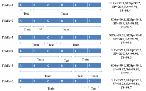
In this work, k-fold cross validation algorithm is used to test the experimental results of the proposed algorithm on the diverse dataset TUG EEG Corpus. From this dataset, 60 EEG signals are obtained (30 EEG signals are belonging to FS case and another 30 EEG signals are belonging to NFS case) and tested with the 6-fold cross validation algorithm, where each iteration contains 6 folds and each fold contains 6 modules and each module contains 10 EEG signals, as illustrated in the Figure 5. At fold 1 (k=1), the signals in A are tested where the signals in the remaining modules are trained. At fold 2 (k=2), the signals in B are tested where the signals in the remaining modules are trained. At fold 3 (k=3), the signals in C are tested where the signals in the remaining modules are trained. At fold 4 (k=4), the signals in D are tested where the signals in the remaining modules are trained. At fold 5 (k=5), the signals in E are tested where the signals in the remaining modules are trained. At fold 6 (k=6), the signals in F are tested where the signals in the remaining modules are trained.
For each fold, the experimental results of the proposed algorithm on the diverse dataset is measured. By taking the average value of all 6 folds, the experimental results on the diverse dataset using the proposed algorithm is similar to the experimental results of the proposed algorithm on BEBA and CHB-MIT datasets.
Figure 5. Cross validation on diverse dataset TUG EEG Corpus using the proposed algorithm
This research work proposes a novel EEGNet deep learning architecture for the detection of FS over NFS EEG signals in order to detect the epileptic seizure. The implementation impact of the WEMD has been analyzed with respect to various existing decomposition methods. This proposed system has been tested with two independent EEG datasets in order to analyze the stability and robustness of the EEG classification process. Finally, the FS can be diagnosed into three severity level classes using the trained EEGNet architecture. The proposed system correctly classifies 1491 FS over 1500 FS on BEBA database and obtains 99.4% FSCR. The proposed system correctly classifies 1191 FS over 1200 FS on CHB-MIT database and obtains 99.2% FSCR. The proposed system correctly classifies 1490 NFS over 1500 NFS on BEBA database and obtains 99.3% NFSCR. The proposed system correctly classifies 1188 FS over 1200 FS on CHB-MIT database and obtains 99% NFSCR. The proposed EEG classification system obtains 99.3% SDSe, 99.1% SDSp, 98.7% SP, 98.9% SA and 98.5% FS on the EEG signals of BEBA database. The proposed EEG classification system obtains 99.1% SDSe, 99.2% SDSp, 98.6% SP, 98.8% SA and 98.7% FS on the EEG signals of CHB-MIT database. Though the present methodologies stated in this work for FS and NFS classification process provided higher and optimum classification rate, these methods have been tested only on dataset signals and hence its stability and robustness have not been analyzed in this work which are identified as the limitations of this paper. The real time EEG signals can be used in future by the proposed methodologies stated in this research work to provide the adaptability of the algorithms to test the stability and robustness performance with large signal count.
The authors would like to thank their friends and colleagues for their constant help and support throughout the study and to obtain the results.
[1] Zabihi, M., Kiranyaz, S., Rad, A.B., Katsaggelos, A.K., Gabbouj, M., Ince, T. (2015). Analysis of high-dimensional phase space via Poincaré section for patient-specific seizure detection. IEEE Transactions on Neural Systems and Rehabilitation Engineering, 24(3): 386-398. https://doi.org/10.1109/TNSRE.2015.2505238
[2] Chowdhury, T.T., Fattah, S.A., Shahnaz, C. (2021). Seizure activity classification based on bimodal Gaussian modeling of the gamma and theta band IMFs of EEG signals. Biomedical Signal Processing and Control, 64: 102273. https://doi.org/10.1016/j.bspc.2020.102273
[3] Natu, M., Bachute, M., Gite, S., Kotecha, K., Vidyarthi, A. (2022). Review on epileptic seizure prediction: Machine learning and deep learning approaches. Computational and Mathematical Methods in Medicine, 2022(1): 7751263. https://doi.org/10.1155/2022/7751263
[4] Usman, S.M., Khalid, S., Akhtar, R., Bortolotto, Z., Bashir, Z., Qiu, H. (2019). Using scalp EEG and intracranial EEG signals for predicting epileptic seizures: Review of available methodologies. Seizure, 71: 258-269. https://doi.org/10.1016/j.seizure.2019.08.006
[5] Shoeibi, A., Ghassemi, N., Khodatars, M., Moridian, P., Alizadehsani, R., et al. (2022). Detection of epileptic seizures on EEG signals using ANFIS classifier, autoencoders and fuzzy entropies. Biomedical Signal Processing and Control, 73: 103417. https://doi.org/10.1016/j.bspc.2021.103417
[6] Truong, N.D., Nguyen, A.D., Kuhlmann, L., Bonyadi, M.R., Yang, J., Ippolito, S., Kavehei, O. (2018). Convolutional neural networks for seizure prediction using intracranial and scalp electroencephalogram. Neural Networks, 105: 104-111. https://doi.org/10.1016/j.neunet.2018.04.018
[7] Tian, X., Deng, Z., Ying, W., Choi, K. S., Wu, D., et al. (2019). Deep multi-view feature learning for EEG-based epileptic seizure detection. IEEE Transactions on Neural Systems and Rehabilitation Engineering, 27(10): 1962-1972. https://doi.org/10.1109/TNSRE.2019.2940485
[8] Gabeff, V., Teijeiro, T., Zapater, M., Cammoun, L., Rheims, S., Ryvlin, P., Atienza, D. (2021). Interpreting deep learning models for epileptic seizure detection on EEG signals. Artificial Intelligence in Medicine, 117: 102084. https://doi.org/10.1016/j.artmed.2021.102084
[9] KR, A.B., Srinivasan, S., Mathivanan, S.K., Venkatesan, M., Malar, B.A., Mallik, S., Qin, H. (2023). A multi-dimensional hybrid CNN-BiLSTM framework for epileptic seizure detection using electroencephalogram signal scrutiny. Systems and Soft Computing, 5: 200062. https://doi.org/10.1016/j.sasc.2023.200062
[10] Shanmugam, S., Dharmar, S. (2023). A CNN-LSTM hybrid network for automatic seizure detection in EEG signals. Neural Computing and Applications, 35(28): 20605-20617. https://doi.org/10.1007/s00521-023-08832-2
[11] Abenna, S., Nahid, M., Bouyghf, H., Ouacha, B. (2022). EEG-based BCI: A novel improvement for EEG signals classification based on real-time preprocessing. Computers in Biology and Medicine, 148: 105931. https://doi.org/10.1016/j.compbiomed.2022.105931
[12] Ahmad, I., Yao, C., Li, L., Chen, Y., Liu, Z., et al. (2024). An efficient feature selection and explainable classification method for EEG-based epileptic seizure detection. Journal of Information Security and Applications, 80: 103654. https://doi.org/10.1016/j.jisa.2023.103654
[13] Kantipudi, M.P., Kumar, N.P., Aluvalu, R., Selvarajan, S., Kotecha, K. (2024). An improved GBSO-TAENN-based EEG signal classification model for epileptic seizure detection. Scientific Reports, 14(1): 843. https://doi.org/10.1038/s41598-024-51337-8
[14] Mathe, M., Mididoddi, P., Battula Tirumala, K. (2023). Electroencephalogram signal classification and artifact removal with deep networks and adaptive thresholding. Journal of Shanghai Jiaotong University (Science), 2023: 1-9. https://doi.org/10.1007/s12204-023-2609-8
[15] Akbari, H., Sadiq, M.T., Rehman, A.U. (2021). Classification of normal and depressed EEG signals based on centered correntropy of rhythms in empirical wavelet transform domain. Health Information Science and Systems, 9: 1-15. https://doi.org/10.1007/s13755-021-00139-7
[16] Hussain, W., Sadiq, M.T., Siuly, S., Rehman, A.U. (2021). Epileptic seizure detection using 1 D-convolutional long short-term memory neural networks. Applied Acoustics, 177: 107941. https://doi.org/10.1016/j.apacoust.2021.107941
[17] The Bern-Barcelona EEG database. https://www.upf.edu/web/ntsa/downloads/-/asset_publisher/xvT6E4pczrBw/content/2012-nonrandomness-nonlinear-dependence-and-nonstationarity-of-electroencephalographic-recordings-from-epilepsy-patients, accessed on 12 Nov., 2024.
[18] Guttag, J. (2010). CHB-MIT scalp EEG database (version 1.0.0). PhysioNet. RRID:SCR_007345. https://doi.org/10.13026/C2K01R, accessed on 12 Nov., 2024.
[19] Zeynali, M., Seyedarabi, H., Afrouzian, R. (2023). Classification of EEG signals using transformer based deep learning and ensemble models. Biomedical Signal Processing and Control, 86: 105130. https://doi.org/10.1016/j.bspc.2023.105130
[20] Si, X., Huang, D., Sun, Y., Huang, S., Huang, H., Ming, D. (2023). Transformer-based ensemble deep learning model for EEG-based emotion recognition. Brain Science Advances, 9(3): 210-223. https://doi.org/10.26599/BSA.2023.905