Utkarsh Dubey*![]() | Raju Barskar
| Raju Barskar![]()
© 2025 The authors. This article is published by IIETA and is licensed under the CC BY 4.0 license (http://creativecommons.org/licenses/by/4.0/).
OPEN ACCESS
Tracking object from various challenges is a key motivation in computer vision and machine learning. It is bit rigorous to fulfill all the challenge with higher level of precision in considering all frames. An immaculate approach is required to build a model for better visual object tracking. It is required to obtain the patterns in each frame for ideal model. Here the research uses Siamese Network and TensorFlow to train and build the model. Siamese Network may contain two or more identical sub-networks that can compare the input and make decision more precise. It is required to pipelining the anchors with positive and negative sources to process the model towards hybrid one for processing the corresponding image. TensorFlow helps to gather the patterns of the objects and recognize it to pertain the same till last frame. Hypothesis is tested with various benchmarks including OTB50, OTB100 and TempleColor128 that pertained better level of precision.
visual object tracking, Siamese Network, TensorFlow, machine learning, OTB50, OTB100, TempleColor128
Visual object tracking is a bit complicated task in computer vision because it involves tracking objects as per the interest with pattern recognition. The motive of object tracking is to project the trajectory of the object along with the position by facing various challenges such as variations in lighting condition, fast motions, getting obstacles over the objects, etc. Tracking algorithm usually works in that manner where it initializes the target object in the very first frame along with its location by using coordinates and other pertinent properties continually in the following frames. It also includes feature extraction, object visualization, pattern following and model prediction. Numerous fields, such as robotics, autonomous navigation, augmented reality, video analysis, surveillance, and human-computer interaction, use visual object tracking extensively [1-3].
It may be used, for example, to guide unmanned aerial vehicles, monitor people and objects in congested areas, analyze sporting events, improve immersive gaming, and provide assistive devices for the blind. Visual object tracking has come a long way in recent years, but it is still a difficult challenge since real-world scenarios are inherently complex and need balancing accuracy, efficiency, and resilience. In order to push the limits of object tracking, researchers are still creating and improving edge tracking algorithms by utilizing developments in deep learning, probabilistic modeling, optimization strategies, and sensor technologies [4].
Several methods are used in visual object tracking to precisely track and identify things throughout a series of frames in a video. Feature extraction techniques, appearance descriptors or keypoints, are commonly employed in these procedures to extract unique attributes from the target object. Motion estimation techniques compute the movement of an item in between frames, enabling placement that is predicted. To capture the item's spatial extent, object representation methods like bounding boxes or pixel-wise masks are used. Similarity metrics assess how an object appears or is composed differently in different frames. To ensure stable and dependable tracking performance, tracking algorithms frequently include techniques for managing occlusions, scale changes, and other difficulties that are frequently encountered in real-world circumstances [5]. The compact visibility can observe several difficulties that work faces during tracking an object using pattern recognition or the features present in the image. It is also required to find out the background of the image to properly segment the foreground for better precision and accuracy.
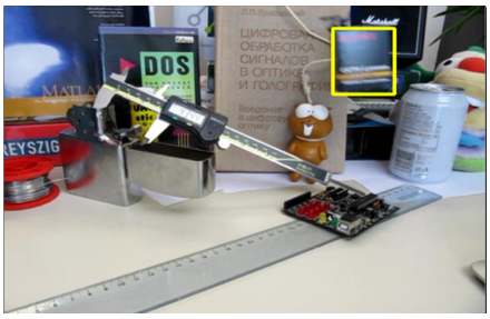
Figure 1 shows a desk with gadgets, where a yellow box highlights one object to demonstrate object tracking.
TensorFlow makes it possible to use deep learning-based algorithms, which makes visual tracking easier. First, target objects for tracking are defined by tagged datasets of pictures or videos. TensorFlow provides a range of pre-trained models, such as SSD and Faster R-CNN, or uses its high-level APIs, such as TensorFlow Keras to enable the development of bespoke models. The prepared datasets are used to train these models, improving their capacity to forecast bounding boxes around tracked objects with precision. The trained models analyze fresh frames and produce predictions for object positions during inference. These predictions can be improved by post-processing methods like smoothing trajectories or removing false positives. Ultimately, the bounding boxes or monitored item coordinates are included into more expansive systems for further examination or utilization.
Figure 1. Visual object tracking [6]
Li et al. [7] presented a network that uses the MA-Dual technique for object tracking and analyzes patterns across frames by using a spatial transient approach. Throughout the whole dataset, the approach extracts structural information using 3D convolutional processing. However, in certain datasets, issues like motion blur and low resolutions make reliable object identification difficult. varied data highlighting under varied brightness circumstances may cause variations in system performance. Comprehensive experiments using UAV123, OTB benchmarks, VOT, and TC128 datasets show the resilience of the approach. Findings show that tracking performance is promising, particularly when managing difficult circumstances including deformation, size variation, and lighting variations.
Zheng et al. [8] presented the Gaussian Process Regression Based Tracker (GPRT), a conventional tracking strategy that uses part tricks and removes boundary effects. The authors improved the performance of GPRT by introducing two effective updating strategies. Analyses performed on the OTB-2013 and OTB-2015 datasets demonstrate that GPRT outperforms trackers using hand-crafted features, with mean overlap accuracy of 84.1% and 79.2%, respectively. By utilizing Gaussian Regression Processes in visual tracking, GPRT presents a unique tracking solution that doesn't require complex add-ons. GPRT not only fully removes boundary effects but also efficiently utilizes the part trick compared to all other CF trackers. The authors also present two unique and effective GPRT updating methods. Two benchmark datasets, OTB-2013 and OTB-2015, with more than 100 films featuring a variety of challenges—birds, bolts, boxes, automobiles, bikers, blurred bodies, football, human, dudek, david, crowds, and more—are used for extensive testing.
Danelljan et al. [9] presented a probabilistic regression framework for tracking in which, given an input picture, the network predicts the restricted probability density of the destination state. The system's architecture is particularly capable of handling noise that results from vague annotations and unclear assignments. The Kullback-Leibler divergence is minimized in order to train the regression network. The framework not only enables a probabilistic representation of the output when used for tracking, but it also greatly enhances performance. On six datasets, the system's tracker achieves a new benchmark with an AUC of 59.8% on LaSOT and a Success rate of 75.8% on TrackingNet.
Chen and Tao [10] suggested a convolutional network-based regression technique for monitoring moving objects. Edge regression is used by the system to extract textures and object patterns for tracking. Furthermore, it combines layered convolutional methods with a backpropagation model. To capture the object's integration features, each layer in the DCF model is customized or trained using a variety of viewpoints. The object tracking system addresses a range of difficulties and sizes by means of repeated iterations and backpropagations. With just one convolutional layer, our technique offers a unique way to comfortably simulate regression in visual tracking.
Millan et al. [11] presented a system for multi-target tracking based on recurrent neural networks (RNNs), providing a novel solution to a number of issues this job presents. Deducing a changing number of targets over time, keeping a continuous state evaluation for every target that is present, and resolving a discrete combinatorial issue are all necessary for tracking many objects in actual scenarios. Earlier techniques frequently use intricate models that need time-consuming parameter adjustment. The authors provide an end-to-end learning architecture for online multi-target tracking, which differs from conventional methods. They point out that current deep learning techniques are not naturally equipped to address these issues and are not easily transferable to the current job.
Yun et al. [12] presented a system built on a deep reinforcement learning algorithm and suggested a novel activity-driven method for visual tracking using deep convolutional networks. The suggested tracker follows the target item iteratively through successive activities while being restricted by an ADNet. The computational complexity of tracking is greatly decreased by using this activity-driven tracking strategy. Furthermore, partly labeled data may be used with reinforcement learning, which might significantly improve training data generation with little work. The evaluation findings show that the proposed tracker outperforms existing deep network-based trackers using a tracking-by-location method by three times, achieving state-of-the-art performance at 3 frames per second.
Like the methods of other writers, he put out a Deep Reinforcement Learning based architecture. They provide a completely end-to-end technique for visual tracking in films that figures out where a target object's bounding box will be at every frame. Considering tracking as a sequential, dynamic process in which past semantics contain very important information for the future is a crucial realization. They create a model that functions as a recurrent convolutional neural network that interacts with video over time by utilizing this intuition. Long-term tracking performance can be improved by teaching the model tracking rules that concentrate on continuous frame boxes through the use of Reinforcement Learning (RL) methods. Operating at increased frame rates, the suggested tracking algorithm achieves state-of-the-art performance on an existing tracking benchmark.
Henriques et al. [13] presented a method based on Kernelized Correlation Filters that showed how normal picture interpretations may be represented in a methodical manner. They demonstrated that under some circumstances, bit frameworks and subsequent information become circulant, making it possible for the Discrete Fourier Transform (DFT) to diagonalize them and to quickly develop algorithms for handling interpretations. The authors developed cutting-edge trackers that operate at high frame rates and need less code implementation by using this approach to linear and patch-based regression. Expansions of their fundamental methodology are probably advantageous in a number of additional issues. Circulant data has proven useful for a number of methods in detection and video event retrieval since this work's original iteration.
Zheng et al. [14] presented an innovative tracking structure dubbed GPRT, which makes use of Gaussian Regression Processes for visual tracking, and he proposed a system based on the Robust Gaussian algorithm. In contrast to existing CF trackers, GPRT concurrently uses part techniques and removes boundary effects. The authors demonstrated the efficacy of two unique, effective GPRT strategies they proposed. Extensive analyses were carried out on the OTB-2013 and OTB-2015 benchmark datasets, where GPRT surpassed all current trackers.
Li et al. [15] presented a Dual Regression model-based system. The authors presented a dual-regression tracking architecture that consists of a CF module and a discriminative convolutional neural network in their study. By learning to distinguish between the target and background, this tracker becomes more discriminative and uses a fully convolutional network to reduce processing overhead. A CF module works on shallower layers with better spatial resolution to fine-tune the target position since deeper layers of the fully convolutional network preserve less spatial detail. This two-stream approach, which uses a single forward CNN pass to estimate the target location, makes deep trackers more effective. The efficacy and efficiency of the suggested approach are demonstrated by evaluation on three publicly available datasets.
Zhang et al. [16] presented a Support Vector Regression (SVR)-based approach. In order to regulate uncalibrated visual servoing for 3D motion tracking, their article suggests a unique approach. In the picture plane, motion based on PI control is initially used. The visual mapping model is then built using SVR. Finally, the continuous mapping approach is used to provide both planar and three-dimensional motion tracking. When compared to conventional BP neural network techniques for 3D motion visual tracking, SVR proved to have good approximation skills, especially when learning from tiny samples.
Zhang et al. [17] suggested a visual tracking method that takes rank loss, shrinkage loss, and optimum feature training into account. They matched target features using the template technique and adjusted their tracking accordingly. But depending just on template-based techniques could result in less than ideal results because these trackers are frequently restricted to particular objectives and have difficulty handling a variety of datasets. In addition to highlighting the necessity of improving the model by optimizing filters to increase processing time, frame rate, and accuracy, the authors propose upgrading the template using preprocessing techniques. To assess the correctness of the system, Templecolor128 will be used for testing. Compared to traditional approaches, object tracking may be greatly aided by object detection since characteristics or patterns can be tracked more successfully.
New developments in Kernelized Correlation Filter (KCF)-based tracking have attempted to address issues such as limited feature representation occlusion and scale variation. Danelljan et al. [18] suggested a better KCF algorithm that uses the MCMRV criterion to incorporate a multi-scale pyramid and an adaptive template update mechanism. This greatly improves the algorithms robustness against occlusion and scale changes while maintaining a high processing speed appropriate for embedded platforms. Zheng et al. [19] improved tracking performance in dynamic scenes with frequent occlusions by introducing an occlusion-aware KCF tracker that incorporates RGB-D information in 2021. Also, Yadav [20] KCF was improved in 2023 by combining deep features from VGG16 which improved the tracker's performance in visually complex and cluttered environments. Maharani et al. [21] additionally, in 2021 long-term tracking problems were addressed by implementing multi-scale detection and Lab color features which decreased model drift and increased stability over long periods of time.
Improvements in methodology have also been made to Multiple Instance Learning (MIL)-based trackers in an effort to make them more resilient and flexible. Cheong and associates showed how different pooling strategies affect classification and tracking performance by comparing different MIL pooling filters such as max mean, attention and distribution-based approaches [22]. Oner et al. [23] used features like compressive tracking and histogram of oriented gradients (HOG) combined MIL, with a parallel tracking and detection framework, improving the tracker's dependability in challenging scenes. Besides, Xiong et al. [24] assessed MIL in a real-time tracking framework on a Raspberry Pi 3 Model B+ platform, demonstrating that although MIL occasionally provided good accuracy, it had trouble maintaining high frame rates on constrained hardware.
This research proposes a hybrid network based on Siamese and TensorFlow, designed for offline processing with large datasets. The network comprises multiple sub-networks for feature extraction, regression, and classification. By integrating the Siamese Network with TensorFlow, an object detection approach, the feature extraction model is enhanced for improved visual tracking analysis. Unlike previous recognition frameworks that repurpose classifiers or localizers for feature extraction, this model applies features across multiple areas of an image, even when objects are scaled. The system will undergo testing with various datasets and benchmarks, including OTB50, OTB100, and TempleColor128, aiming to achieve higher levels of accuracy.
3.1 Problem definition
Even though visual object tracking has advanced significantly consideration to methods like deep learning regression models and reinforcement learning a number of significant obstacles still exist. Among these are the challenges of preserving robustness in the face of unfavorable circumstances like motion blur, low resolution, fluctuating lighting and object deformation. The real-world applicability of many current methods is limited by their struggles with boundary effects occlusion and generalization across diverse datasets. Furthermore, intricate designs are frequently unsuitable for real-time applications and necessitate extensive tuning. Effective mechanisms to manage long-term dependencies and update models effectively during tracking are also lacking. Tracking accuracy and speed balance is still a big concern which emphasizes the need for more flexible lightweight and dependable tracking systems that can function well in a variety of situations.
3.1.1 Method design
To precisely localize the target object in every frame the suggested method design for visual object tracking combines a lightweight regression framework with a feature extraction module based on Convolutional Neural Networks (CNNs). First input frames undergo preprocessing, which includes normalization and resizing and a region of interest is chosen for effective calculation. Selected CNN layers that strike a balance between semantic richness and spatial detail are used to extract deep features. After that the target bounding box is predicted by a regression-based tracking module. To account for variations in appearance scale and occlusion, an adaptive update strategy uses confidence-based online learning to improve the model. A re-detection mechanism is incorporated for tracking failure recovery and frame-wise predictions are smoothed to improve temporal consistency. Stochastic gradient descent is used to optimize the model after it has been trained using a combination of regression and similarity-based loss functions. Metrics like precision AUC, and success rate are used to assess the model's robustness and real-time capability on benchmark datasets like OTB VOT, and LaSOT.
3.1.2 Experimental validation
To ensure a thorough performance evaluation under a variety of real-world scenarios the proposed visual object tracking system was experimentally validated on well-known benchmark datasets such as OTB-2013 OTB-2015 VOT LaSOT and UAV123. Standard metrics like accuracy success rate intersection over union (IoU) and area under the curve (AUC) were used to gauge the systems performance. To demonstrate gains in robustness, adaptability and tracking accuracy especially in the face of difficult circumstances like motion blur occlusion scale variation and illumination changes a comparative analysis was conducted against a number of cutting-edge trackers. Across sequences with different object classes motion patterns and scene complexities the suggested method continuously outperformed baseline approaches exhibiting superior tracking stability and efficiency while preserving real-time performance with little computational overhead.
3.2 Siamese network
Common applications of the Siamese neural network include object tracking and similarity learning. The fundamental design consists of two similar neural networks with the same topology and weights, often referred to as Siamese twins or twin networks. The Siamese neural network may be represented mathematically in the following way:
Let $f(x ; \theta)$ stands for the function that the neural network learnt, where x is the input and θ is the network's parameters (weights and biases). MThe modelhas two identical networks sharing the same parameters for a Siamese Network. Let's say that the inputs to the first and second networks are represented by the symbols x1 and x2, respectively. The output of each network is a feature vector, denoted as $f\left(x_1 ; \theta\right)$ and $f\left(x_2 ; \theta\right)$ espectively. In other words, the following mathematical representation captures the fundamental structure of a Siamese Neural network:
$f\left(x_1 ; \theta\right)=\operatorname{Net}\left(x_1 ; \theta\right)$ (1)
$f\left(x_2 ; \theta\right)=\operatorname{Net}\left(x_2 ; \theta\right)$ (2)
$S\left(x_1, x_2\right)=$ Similarity $f\left(x_1 ; \theta\right), f\left(x_2 ; \theta\right)$ (3)
where, $f\left(x_1 ; \theta\right)$ is the feature vector of first input with the network parameter $\theta$, similarly for the $f\left(x_2 ; \theta\right) . S\left(x_1, x_2\right)$ is the similarity between the first input vector and the second one.
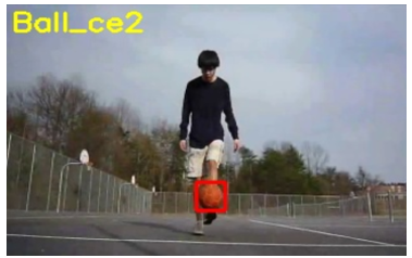
In actuality, depending on the particular job and application, the network design, loss function, and optimization technique may change. Additionally, Siamese Networks are frequently trained for similarity learning tasks using methods like contrastive loss and triplet loss. In order to extract image characteristics, the Siamese Network uses the categorization network, which biases the retrieved features toward semantic information. SiameseRPN++ uses ResNet as its feature extraction backbone network. The findings of the experiment confirm that various channels respond differently to distinct object categories, suggesting that deep features can capture semantic information associated with object prejudice. The Siamese Network's dual-branch structure allows it to interpret input picture data in a different way, producing characteristics that take various dimensions, such as channel and space, into account. By using the attention mechanism to filter visual data, the network is able to determine the object's significance during feature extraction, highlighting target features that are pertinent to the tracking job and ignoring background information. The most adorable feature of Siamese Network is offline learning approach. It trains the model in offline mode and test in the same manner. The template branch and the detection branch are the two branches that make up the Siamese tracker. While the detection branch examines the target image patch from the current frame, the template branch receives the target image patch from the previous frame as input. To track an object, first of all, it is required to preprocess the image using smart filters and localize the image by inputting the target object in the very first frame. Figure 2 illustrates the box marks target object initialization in object tracking selecting the ball as the focus to follow in the video.
Figure 2. Target object initialization
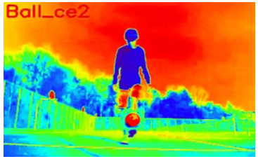
Figure 3. Color mapping of target feature object
The process of extracting features began when the target object was established. Using a set of pixels with comparable spectral, spatial, and/or textural qualities, an object (or segment) is used in feature extraction, an object-based method for classifying images. Figure 3 shows the color mapping highlights the ball’s features to initialize it as the tracking target.
On the other hand, conventional classification techniques are pixel-based, categorizing images based on the spectral information of individual pixels.
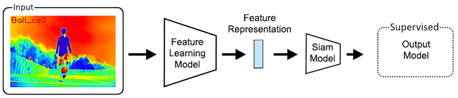
Figure 4. Task specific model training
Once the feature extraction has been done, then feature training will be started, and with the help of Siamese Network; task-specific training will be accomplished and generate the output model. Figure 4 illustrates task-specific model training in object tracking.
3.3 TensorFlow
For object identification tasks, TensorFlow is a powerful tool with an extensive ecosystem of models and tools. Choosing an appropriate model architecture, such as Faster R-CNN, SSD, or YOLO, which each have their trade-offs between speed and accuracy, is usually the first step in the process.
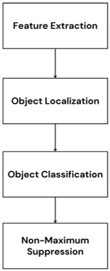
Convolutional neural networks (CNNs) are used by these designs to forecast bounding boxes and class labels for objects that are recognized, as well as to extract characteristics from input photos. Using hierarchical features that capture semantic information about the objects in the image, CNNs process the input image. Convolutional and pooling layers, which gradually decrease the spatial dimensions while increasing the depth of feature maps, are commonly used to achieve this. The model predicts bounding boxes, or coordinates, that closely surround items of interest inside the picture once features are retrieved. Figure 5 shows the main steps in TensorFlow object detection: extracting features, finding and classifying objects, then filtering results. Regressing the coordinates of a group of predetermined anchor boxes to better suit the position of the item is a common method for doing this. At the same time, the model classifies objects by giving each bounding box a class probability that indicates how likely it is to include a certain item category. In order to compute class probabilities, this is often accomplished using extra convolutional layers and a softmax activation function. Non-Maximum Suppression is used to filter out overlapping bounding boxes with lower confidence ratings in order to get rid of redundant detections. This guarantees the retention of just the most certain detections. Three phases are usually included in the object detection operation:
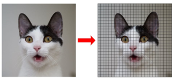
(a) The way that the input is divided into manageable chunks. Figure 6 demonstrates image segmentation: the grid divides the cat photo into distinct regions, helping separate and analyze parts of the image for tasks like object recognition. The whole image is covered by the extensive collection of bounding boxes, as shown.
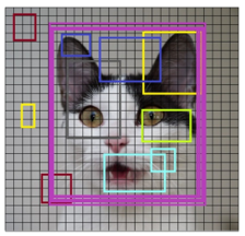
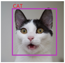
(b) For each segmented rectangular area, feature extraction is conducted to determine whether the rectangle contains a valid object. Each box shows a region where features are extracted for later recognition or tracking is presented in Figure 7. Figure 8 depicts Non-Maximum Suppression merges overlapping detection boxes into one, creating a single rectangle around the cat.
Non-Maximum Suppression creates a single boundary rectangle by joining overlapping boxes.
Figure 5. Visual object detection in TensorFlow
Figure 6. Segmentation of an image
Figure 7. Feature extraction of all boxes
Figure 8. Object detection using non-max suppression
3.4 Architecture of Siamese Network
Siamese Networks are a subclass of networks defined by the use of two sub-networks that are exactly the same for one-shot classification tasks. Even though these sub-networks analyze distinct inputs, they retain the same designs, parameters, and weights. Siamese Networks learn a similarity function, in contrast to typical CNNs that are trained on large datasets to predict various classes. They can distinguish between classes with less data thanks to this feature, which makes them quite effective for one-shot classification tasks. These networks are frequently able to categorize pictures effectively with only one sample thanks to their amazing feature. Instead of using a lot of labeled data for training as in the standard technique, few-shot learning trains models to make predictions using only a limited number of instances. When it becomes difficult or expensive to gather large amounts of labeled data, the value of few-shot learning becomes clear. Few-shot models may produce predictions with little input sometimes even from a single example because of its design, which captures the intricacies seen in a tiny sample size. This feature is made possible by several design processes including Siamese Networks, Meta-learning, and related techniques. With the help of these frameworks, the model is able to derive insightful data representations and apply them successfully to new, untested samples.
The goal of the differencing layer is to draw attention to the differences between dissimilar pairs while highlighting the commonalities between inputs. The Euclidean Distance function is employed to do:
Distance $\left(x_1, x_2\right)=\left\|\mathrm{f}\left(x_1\right)-\mathrm{f}\left(x_2\right)\right\|_2$ (4)
Here, x1 and x2 represent the two inputs, Encoding (x₁) and Encoding(x2) denote the output of the encoding function, and Distance represents the distance function. The entropy loss can be encountered as:
$-(y \log (p)+(1-y) \log (1-p))$ (5)
where,
y represents the true label,
p represents the predicted probability
$K(i, j)=\frac{\sum_{x=1}^N \sum_{y=1}^N(x, y) \times T(x, y)}{\sqrt{\sum_{x=1}^N \sum_{y=1}^N[S(x, y)]^2} \sqrt{\sum_{x=1}^N \sum_{y=1}^N[T(x, y)]^2}}$ (6)
where,
T(x,y) denotes the template image,
S(x,y) represents the search region of the target, and
K indicates the height and width of the data.
The response map is obtained by using a fully-convolutional Siamese Network, as shown in the flow chart of the Siamese framework. The re-detection network is initiated if the secondary peak in this map is more than 0.75 times the size of the main peak.
3.5 Process model
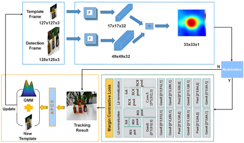
To maximize input quality, the system first gathers frames for preprocessing. The networks are obtained and loaded to recognize objects based just on their appearance once all preprocessing activities have been completed. Figure 9 shows a Siamese network architecture for object detection, where parallel networks compare a template and a detection frame to localize and track the target object.
Figure 9. Object detection Siamese Network architecture
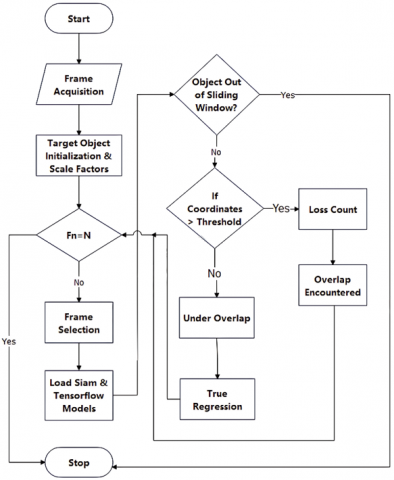
After that, an additional network is utilized for effective object tracking. The system makes use of two distinct strategies that are well-known for their effectiveness in tracking and object identification, which helps to improve the regression model. This minimizes overlap counts and increases frame rate per second while maintaining excellent system efficiency. Figure 10 represented the proposed flow chart.
Figure 10. Proposed flow chart
|
Algorithm 1: Siamese & TensorFlow Algorithm |
|
Initialization Input: Frames Output: (X, Y) Coordinates Step 1. Initialize: - Input the first frame of the dataset. Step 2. Convert: - Convert the RGB image to grayscale. Step 3. Setup: - Define the target area or object according to the dataset. Step 4. Frame Sequences: - Establish frame sequences {Xt}T, where X1 represents the initial frame. Step 5. Model Loading: - Load the Siamese and TensorFlow models. Step 6. Iterate: - For each iteration (I) from 1 to N: - Search for the target object in the frames. - If the detection confidence exceeds the threshold value: - Increment the count for overlapping detections. - Else: - Increment the count for accurately regressed objects. Step 7. Extraction: - Extract coordinates: Cx (width), Cy (height), X, and Y (coordinates of the target object). Step 8. Comparison: - Compare extracted coordinates with ground truth. Step 9. Accuracy Calculation: - Compute system accuracy using counts of loss and true regression. Step 10. End: - Terminate the algorithm |
First, frames from a dataset are entered and converted from RGB to grayscale using the Siamese Network and TensorFlow technique. After that, it creates frame sequences and specifies the target region or object in accordance with the dataset criteria. In order to start the detection procedure, the algorithm loads the TensorFlow and Siamese Network models. It looks for the target item inside the frames throughout each cycle. It counts successfully regressed items and increases the count for overlapping detections if the detection confidence is greater than a predetermined threshold. The target object's width, height, and (x, y) coordinates are extracted by the method. It then evaluates accuracy by contrasting these extracted coordinates with the ground truth. Lastly, it uses counts of loss and true regression to calculate the accuracy of the system before terminating the algorithm. To guarantee efficient object tracking the Siamese Network and TensorFlow hybrid tracking model was put into practice with particular training setups and parameters. To filter and improve detection results Non-Maximum Suppression (NMS) was applied with a confidence threshold of 0. 5 and an IoU threshold of 0. 4. The Adam optimizer was used to optimize the Contrastive Loss function over 50 epochs with a batch size of 32. The learning rate was set at 1e-4. It used a modified AlexNet as the feature embedding backbone and standardized the input images to 127×127 for the exemplar (template) and 255×255 for the search region. The algorithmic flow was made more understandable by adding a pseudocode representation that detailed the steps involved from feature extraction and similarity calculation to score thresholding and final bounding box selection. All of these specifics improve the suggested methods transparency and reproducibility.
TensorFlow version 2.12 and Python 3.10 were used for the implementation, which was run on a hardware configuration that included an Intel Core i7 processor 10GB VRAM, 16 GB system’s RAM, and an NVIDIA RTX 3060 GPU. Effective model evaluation and training were guaranteed by this setup. The model was trained with a learning rate of 1e-4 a batch size of 32 and for a total of 50 epochs in order to support reproducibility. The training parameters and other hardware and software specifics are documented for clarity and to enable others to precisely reproduce the experimental conditions. The suggested tracker is assessed using both qualitative and quantitative methods. Several tests are performed on a collection of twenty-three chosen movies from three well-known datasets: OTB-50, OTB-100, and Temple Colour-128. A variety of visual difficulties may be seen in these films, such as cluttering, out-of-plane rotation, occlusion, scale fluctuations, deformation, rapid motion, and motion blur. For experimental validation the OTB-50 OTB-100 and TC128 datasets were chosen based on their usage in the base paper, guaranteeing consistency and comparability of findings. These datasets are well-known within the visual tracking community and offer a variety of tracking scenarios that are crucial for assessing the robustness and performance of tracking algorithms.
OTB-50 and OTB-100 are perfect for evaluating short-term tracking abilities under a variety of difficult circumstances because they provide sequences with annotated attributes like occlusion illumination variation scale changes and fast motion. By adding increasingly intricate and cluttered environments, TC128 expands on this assessment and puts the algorithms flexibility and accuracy to the test. We guarantee a fair and straightforward performance comparison by utilizing the same datasets as the base study, confirming the efficacy of the suggested approach in comparable experimental conditions. The coordinates from the suggested system are used to calculate the results, which are then compared to the ground truth values. Two benchmarks, OTB50, OTB100, and TempleColor128, each including several films with thousands of frames, are used to assess the suggested method. Specific problems that align with the benchmark qualities are presented in each video. Eleven characteristics are commonly employed to evaluate the correctness of the system, such as overflow and accurate object detection at every frame. If the bounding boxes fall beyond the window or surpass a threshold value, an error occurs that reduces accuracy. Frame per Second (FPS) has been measured to obtain the execution time. Success and precision are two parameters through which results have been computed accordingly.
Success is evaluated on the basis of how current bounding box overlaps with the ground truth bounding box. There is a parameter Intersection over Union (IoU) that lies between the predicted outcome and the ground truth.
$ Success =\frac{Area \, of \, Overlap}{Area \, of \, Union}$
IoU is encountered when it exceeds the threshold value i.e. 20 pixels. Whereas precision is calculated on the basis of the center location of the bounding box as well as the ground truth. There is only a difference is the threshold where 50 pixels are considered for precision.
$Precison=\frac{Number \, of \, frames<threshold}{Total \, number \, of \, frames}$
If IoU ≥ 0.5, then 0.5 is considered as the ground truth threshold. Each video contains a total number of frames, and if the bounding box fails to track the target object, the frames in which the target is lost are counted as loss frames.
$Accuracy=\frac{Total \, Number \, of \, Frames-Total \, Predicted \, Loss \, Frames}{Total \, Number \, of \, Frames} \times 100 \%$
$ Loss Count =100- Predicted \, Accuracy \%$
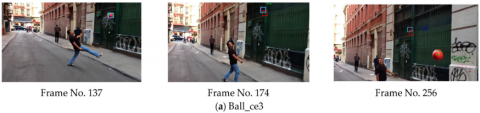
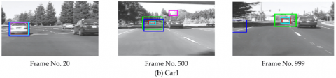
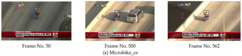
Figure 11 shows sample frames from tracking datasets (OTB-50, OTB-100, Temple Colour-128), with colored boxes marking tracked objects in each scene.
Figure 11. Selected videos from OTB-50, OTB-100, and Temple Colour-128 datasets
Tables 1-6 present the recorded performance metrics across three datasets. Tables 1 and 2 show the accuracy and loss count for OTB-50, respectively. Tables 3 and 4 provide the corresponding metrics for OTB-100, while Tables 5 and 6 detail the accuracy and loss count for TC-128.
Table 1. Recorded accuracy of OTB-50
|
Datasets |
Accuracy |
FPS |
Datasets |
Accuracy |
FPS |
|
Basketball |
100.00 |
285.0 |
Human3 |
100.00 |
127.1 |
|
Biker |
100.00 |
280.5 |
Human4 |
54.52 |
295.5 |
|
Bird1 |
46.43 |
271.1 |
Human6 |
93.15 |
243.6 |
|
BlurBody |
99.40 |
206.9 |
Human9 |
100.00 |
300.4 |
|
BlurCar2 |
85.62 |
248.9 |
Ironman |
80.77 |
286.0 |
|
BlurFace |
64.42 |
233.0 |
Jump |
96.69 |
275.5 |
|
BlurOwl |
98.57 |
293.0 |
Jumping |
100.00 |
301.7 |
|
Bolt |
100.00 |
299.3 |
Liqour |
59.95 |
184.1 |
|
Box |
99.05 |
172.3 |
Matrix |
89.80 |
262.1 |
|
Car1 |
100.00 |
235.8 |
MotorRollig |
95.00 |
272.3 |
|
Car4 |
100.00 |
290.4 |
Panda |
100.00 |
239.9 |
|
CarDark |
100.00 |
304.7 |
RedTeam |
100.00 |
193.4 |
|
CarScale |
96.80 |
269.4 |
Shaking |
100.00 |
294.9 |
|
ClifBar |
96.40 |
297.8 |
Singer2 |
81.06 |
298.7 |
|
Couple |
100.00 |
278.8 |
Skating1 |
89.13 |
290.6 |
|
Crowds |
100.00 |
291.1 |
Skating2 |
72.13 |
269.3 |
|
David |
81.09 |
263.0 |
Skiing |
100.00 |
263.0 |
|
Deer |
100.00 |
237.9 |
Soccer |
92.59 |
260.0 |
|
Diving |
98.60 |
284.2 |
Surfur |
100.00 |
300.8 |
|
DragonBaby |
89.19 |
270.3 |
Sylvester |
100.00 |
206.7 |
|
Dudek |
99.56 |
169.8 |
Tiger2 |
87.33 |
262.3 |
|
Football |
55.15 |
248.7 |
Trellis |
100.00 |
294.7 |
|
Freeman4 |
94.31 |
301.8 |
Walking |
100.00 |
289.7 |
|
Girl |
100.00 |
302.3 |
Walking2 |
100.00 |
302.9 |
|
|
|
|
Woman |
97.65 |
301.7 |
|
Mean |
|
91.72 |
|
||
Table 2. Recorded loss count of OTB-50
|
Datasets |
Overlap |
Datasets |
Overlap |
|
Basketball |
0.00 |
Human3 |
0.00 |
|
Biker |
0.00 |
Human4 |
45.48 |
|
Bird1 |
53.57 |
Human6 |
6.85 |
|
BlurBody |
0.60 |
Human9 |
0.00 |
|
BlurCar2 |
14.38 |
Ironman |
19.23 |
|
BlurFace |
35.58 |
Jump |
3.31 |
|
BlurOwl |
1.42 |
Jumping |
0.00 |
|
Bolt |
0.00 |
Liqour |
40.05 |
|
Box |
0.95 |
Matrix |
10.20 |
|
Car1 |
0.00 |
MotorRolling |
5.00 |
|
Car4 |
0.00 |
Panda |
0.00 |
|
CarDark |
0.00 |
RedTeam |
0.00 |
|
CarScale |
3.20 |
Shaking |
0.00 |
|
ClifBar |
3.61 |
Singer2 |
18.94 |
|
Couple |
0.00 |
Skating1 |
10.87 |
|
Crowds |
0.00 |
Skating2 |
27.87 |
|
David |
18.91 |
Skiing |
0.00 |
|
Deer |
0.00 |
Soccer |
7.41 |
|
Diving |
1.40 |
Surfur |
0.00 |
|
DragonBaby |
10.81 |
Sylvester |
0.00 |
|
Dudek |
0.44 |
Tiger2 |
12.67 |
|
Football |
44.85 |
Trellis |
0.00 |
|
Freeman4 |
5.69 |
Walking |
0.00 |
|
Girl |
0.00 |
Walking2 |
0.00 |
|
|
|
Woman |
2.35 |
|
Mean |
8.28 |
||
Table 3. Recorded accuracy of OTB-100
|
Datasets |
Accuracy |
FPS |
Datasets |
Accuracy |
FPS |
|
Bird2 |
100.00 |
267.1 |
Freeman1 |
100.00 |
294.9 |
|
BlurCar1 |
99.05 |
270.0 |
Freeman3 |
100.00 |
296.5 |
|
BlurCar3 |
100.00 |
294.0 |
Girl2 |
46.30 |
194.2 |
|
BlurCar4 |
93.62 |
239.3 |
Gym |
100.00 |
256.1 |
|
Board |
60.17 |
223.2 |
Human2 |
94.67 |
125.5 |
|
Bolt2 |
69.10 |
302.6 |
Human5 |
100.00 |
280.2 |
|
Boy |
100.00 |
303.3 |
Human7 |
100.00 |
293.7 |
|
Car2 |
100.00 |
253.2 |
Human8 |
100.00 |
264.7 |
|
Car24 |
100.00 |
174.5 |
Jogging |
100.00 |
283.0 |
|
Coke |
93.75 |
285.2 |
KiteSurf |
100.00 |
271.3 |
|
Coupon |
41.25 |
291.0 |
Lemming |
93.54 |
149.4 |
|
Crossing |
100.00 |
286.0 |
Man |
100.00 |
291.4 |
|
Dancer |
100.00 |
265.0 |
Mhyang |
100.00 |
196.9 |
|
Dancer2 |
100.00 |
273.5 |
MountainBike |
100.00 |
290.5 |
|
David2 |
100.00 |
303.8 |
Rubik |
97.59 |
117.8 |
|
David3 |
98.79 |
287.1 |
Singer1 |
100.00 |
252.1 |
|
Dog |
87.50 |
275.3 |
Skater |
100.00 |
264.0 |
|
Dog1 |
41.02 |
162.0 |
Skater2 |
96.06 |
270.6 |
|
Doll |
97.60 |
164.8 |
Subway |
100.00 |
296.9 |
|
FaceOcc1 |
41.83 |
239.8 |
Suv |
100.00 |
289.7 |
|
FaceOcc2 |
76.72 |
260.8 |
Tiger1 |
99.43 |
255.6 |
|
Fish |
100.00 |
284.6 |
Toy |
98.51 |
285.2 |
|
Fleetface |
66.10 |
217.7 |
Trans |
50.00 |
191.9 |
|
Football1 |
100.00 |
267.6 |
Twinnings |
99.79 |
295.1 |
|
|
|
|
Vase |
88.76 |
270.4 |
|
Mean |
|
90.43 |
|
||
Table 4. Recorded loss count of OTB-100
|
Datasets |
Overlap |
Datasets |
Overlap |
|
Bird2 |
0.00 |
Freeman1 |
0.00 |
|
BlurCar1 |
0.948 |
Freeman3 |
0.00 |
|
BlurCar3 |
0.00 |
Girl2 |
53.69 |
|
BlurCar4 |
6.38 |
Gym |
0.00 |
|
Board |
39.82 |
Human2 |
5.33 |
|
Bolt2 |
30.90 |
Human5 |
0.00 |
|
Boy |
0.00 |
Human7 |
0.00 |
|
Car2 |
0.00 |
Human8 |
0.00 |
|
Car24 |
0.00 |
Jogging |
0.00 |
|
Coke |
6.25 |
KiteSurf |
0.00 |
|
Coupon |
58.75 |
Lemming |
6.45 |
|
Crossing |
0.00 |
Man |
0.00 |
|
Dancer |
0.00 |
Mhyang |
0.00 |
|
Dancer2 |
0.00 |
MountainBike |
0.00 |
|
David2 |
0.00 |
Rubik |
2.41 |
|
David3 |
1.21 |
Singer1 |
0.00 |
|
Dog |
12.50 |
Skater |
0.00 |
|
Dog1 |
58.98 |
Skater2 |
3.94 |
|
Doll |
2.40 |
Subway |
0.00 |
|
FaceOcc1 |
58.17 |
Suv |
0.00 |
|
FaceOcc2 |
23.28 |
Tiger1 |
0.57 |
|
Fish |
0.00 |
Toy |
1.49 |
|
Fleetface |
33.90 |
Trans |
50.00 |
|
Football1 |
0.00 |
Twinnings |
0.21 |
|
|
|
Vase |
11.24 |
|
Mean |
9.57 |
||
Table 5. Recorded accuracy of TC-128
|
Datasets |
Accuracy |
FPS |
Datasets |
Accuracy |
FPS |
|
Airport_ce |
62.16216 |
121.7 |
Kite_ce3 |
100 |
302.8 |
|
Baby_ce_gt |
100 |
294.4 |
Kobe_ce |
100 |
258.4 |
|
Badminton_ce1 |
100 |
304.3 |
Lemming |
100 |
141.1 |
|
Badminton_ce2 |
100 |
251.8 |
Liquor |
100 |
180.9 |
|
Ball_ce1 |
71.86701 |
261.2 |
Logo_ce |
100 |
270.6 |
|
Ball_ce2 |
100 |
304.0 |
Matrix |
74.19355 |
274.7 |
|
Ball_ce3 |
99.6337 |
252.8 |
Messi_ce |
58.00 |
298.5 |
|
Ball_ce4 |
81.07527 |
304.6 |
Michaeljackson_ce |
100 |
127.5 |
|
Basketball |
100 |
268.4 |
Microphone_ce1 |
72.51908 |
284.9 |
|
Basketball_ce1 |
100 |
300.9 |
Microphone_ce2 |
100 |
288.8 |
|
Basketball_ce2 |
98.24561 |
299.2 |
Motorbike_ce |
100 |
283.8 |
|
Basketball_ce3 |
89.14027 |
290.5 |
MotorRolling |
100 |
269.6 |
|
Bee_ce |
73.68421 |
270.4 |
MountainBike |
71.95122 |
298.2 |
|
Bicycle |
100 |
296.2 |
Panda |
100 |
298.4 |
|
Bike_ce1 |
100 |
271.6 |
Plane_ce2 |
84.6473 |
301.8 |
|
Bike_ce2 |
100 |
268.0 |
Plate_ce1 |
87.09677 |
279.5 |
|
Biker |
66.85083 |
259.4 |
Plate_ce2 |
100 |
286.1 |
|
Bikeshow_ce |
94.5544 |
286.0 |
Pool_ce1 |
100 |
300.9 |
|
Bird |
91.43646 |
258.1 |
Pool_ce2 |
100 |
294.5 |
|
Board |
88.00 |
242.9 |
Pool_ce3 |
100 |
290.9 |
|
Boat_ce1 |
78.70968 |
290.2 |
Railwaystation_ce |
14.51613 |
232.4 |
|
Boat_ce2 |
94.44444 |
297.6 |
Ring_ce |
71.91283 |
298.8 |
|
Bolt |
100 |
301.2 |
Sailor_ce |
100 |
301.6 |
|
Boy |
69.51567 |
305.0 |
Shaking |
81.8408 |
295.4 |
|
Busstation_ce1 |
100 |
288.1 |
Singer_ce1 |
100 |
287.6 |
|
Busstation_ce2 |
95.6044 |
294.2 |
Singer_ce2 |
83.64486 |
171.1 |
|
CarDark |
100 |
309.9 |
Singer1 |
90.32258 |
276.9 |
|
CarScale |
100 |
287.7 |
Singer2 |
85.75499 |
300.3 |
|
Carchasing_ce1 |
100 |
236.4 |
Skating_ce1 |
73.49727 |
203.2 |
|
Carchasing_ce3 |
100 |
313.5 |
Skating_ce2 |
70.66015 |
95.70 |
|
Carchasing_ce4 |
100 |
301.8 |
Skating1 |
74.19355 |
292.7 |
|
Charger_ce |
100 |
91.3 |
Skating2 |
90.75 |
273.5 |
|
Coke |
69.46309 |
292.6 |
Skiing |
93.11828 |
274.1 |
|
Couple |
100 |
286.4 |
Skiing_ce |
100 |
168.3 |
|
Crossing |
98.57143 |
278.1 |
Skyjumping_ce |
80.43011 |
250.7 |
|
Cup |
100 |
295.6 |
Soccer |
100 |
284.3 |
|
Cup_ce |
100 |
290.1 |
Spiderman_ce |
83.92857 |
227.0 |
|
David |
71.30178 |
272.8 |
Subway |
74.43182 |
284.3 |
|
David3 |
74.19355 |
293.9 |
Suitcase_ce |
61.71429 |
247.9 |
|
Deer |
100 |
227.4 |
Sunshade |
81.52174 |
303.7 |
|
Diving |
84.50704 |
279.3 |
SuperMario_ce |
98.83721 |
253.3 |
|
Doll |
93.93939 |
151.5 |
Surf_ce1 |
92.44186 |
204.6 |
|
Eagle_ce |
100 |
290.7 |
Surf_ce2 |
94.05941 |
119.6 |
|
Electricalbike_ce |
50.00 |
232.3 |
Surf_ce3 |
78.26087 |
246.9 |
|
Face_ce |
100 |
139 |
Surf_ce4 |
69.17563 |
215.1 |
|
Face_ce |
75.48387 |
224.1 |
TableTennis_ce |
74.81481 |
308.5 |
|
Fish_ce1 |
35.13514 |
225.2 |
Tennis_ce1 |
89.39394 |
252.3 |
|
Fish_ce2 |
95.05376 |
286.7 |
Tennis_ce2 |
76.65198 |
238.8 |
|
FaceOcc1 |
100 |
276.5 |
Tennis_ce3 |
97.70492 |
243.8 |
|
Football1 |
98.27957 |
270.1 |
TennisBall_ce |
83.82353 |
291.0 |
|
Girl |
91.35802 |
299.3 |
Thunder_ce |
95.13889 |
296.2 |
|
Girlmov |
100 |
108 |
Tiger1 |
100 |
242.3 |
|
Guitar_ce1 |
93.97849 |
284.2 |
Tiger2 |
97.45763 |
280.8 |
|
Guitar_ce2 |
100 |
230.1 |
Torus |
98.63014 |
297.3 |
|
Gym |
79.8722 |
275.8 |
Toyplane_ce |
100 |
252.7 |
|
Hand |
100 |
275.4 |
Trellis |
78.2716 |
305.2 |
|
Hand_ce1 |
69.67213 |
203.9 |
Walking |
97.2043 |
295.6 |
|
Hand_ce2 |
99.25187 |
286.6 |
Walking2 |
100 |
293.0 |
|
Hurdle_ce1 |
100 |
237.7 |
Woman |
96.12903 |
310.7 |
|
Hurdle_ce2 |
60.00 |
293.8 |
Yo-yos_ce1 |
100 |
293.4 |
|
Iceskater |
100 |
261.5 |
Yo-yos_ce2 |
88.93617 |
286.1 |
|
Ironman |
100 |
284.3 |
Yo-yos_ce3 |
82.15859 |
285.7 |
|
Jogging [1] |
96.38554 |
292.5 |
|
|
|
|
Jogging [2] |
75.57003 |
286.6 |
|
|
|
|
Juice |
74.59283 |
301.9 |
|
|
|
|
Kite_ce1 |
100 |
307.2 |
|
|
|
|
Kite_ce2 |
100 |
309.7 |
|
|
|
|
Mean |
|
89.07961 |
|
||
Table 6. Recorded loss count of TC-128
|
Datasets |
Overlap |
Datasets |
Overlap |
|
Airport_ce |
37.83784 |
Kite_ce3 |
0 |
|
Baby_ce_gt |
0 |
Kobe_ce |
0 |
|
Badminton_ce1 |
0 |
Lemming |
0 |
|
Badminton_ce2 |
0 |
Liquor |
0 |
|
Ball_ce1 |
28.13299 |
Logo_ce |
25.80645 |
|
Ball_ce2 |
0 |
Matrix |
42 |
|
Ball_ce3 |
0.3663 |
Messi_ce |
0 |
|
Ball_ce4 |
18.92473 |
Michaeljackson_ce |
27.48092 |
|
Basketball |
0 |
Microphone_ce1 |
0 |
|
Basketball_ce1 |
0 |
Microphone_ce2 |
0 |
|
Basketball_ce2 |
1.75439 |
Motorbike_ce |
0 |
|
Basketball_ce3 |
10.85973 |
MotorRolling |
28.04878 |
|
Bee_ce |
26.31579 |
MountainBike |
0 |
|
Bicycle |
0 |
Panda |
15.3527 |
|
Bike_ce1 |
0 |
Plane_ce2 |
12.90323 |
|
Bike_ce2 |
0 |
Plate_ce1 |
0 |
|
Biker |
33.14917 |
Plate_ce2 |
0 |
|
Board |
12 |
Pool_ce1 |
0 |
|
Boat_ce1 |
21.29032 |
Pool_ce2 |
85.48387 |
|
Boat_ce2 |
5.55556 |
Pool_ce3 |
28.08717 |
|
Bolt |
0 |
Railwaystation_ce |
0 |
|
Boy |
30.48433 |
Ring_ce |
18.1592 |
|
Busstation_ce1 |
0 |
Sailor_ce |
0 |
|
Busstation_ce2 |
4.3956 |
Shaking |
16.35514 |
|
CarDark |
0 |
Singer_ce1 |
9.67742 |
|
CarScale |
0 |
Singer_ce2 |
14.24501 |
|
Carchasing_ce1 |
0 |
Singer1 |
26.50273 |
|
Carchasing_ce3 |
0 |
Singer2 |
29.33985 |
|
Carchasing_ce4 |
0 |
Skating_ce1 |
25.80645 |
|
Charger_ce |
0 |
Skating_ce2 |
9.25 |
|
Coke |
30.53691 |
Skating1 |
6.88172 |
|
Couple |
0 |
Skating2 |
0 |
|
Crossing |
1.42857 |
Skiing |
19.56989 |
|
Cup |
0 |
Skiing_ce |
0 |
|
Cup_ce |
0 |
Skyjumping_ce |
16.07143 |
|
David |
28.69822 |
Soccer |
25.56818 |
|
David3 |
25.80645 |
Spiderman_ce |
38.28571 |
|
Deer |
0 |
Subway |
18.47826 |
|
Diving |
15.49296 |
Suitcase_ce |
1.16279 |
|
Doll |
6.06061 |
Sunshade |
7.55814 |
|
Eagle_ce |
0 |
SuperMario_ce |
5.94059 |
|
Electricalbike_ce |
50 |
Surf_ce1 |
21.73913 |
|
Face_ce |
0 |
Surf_ce2 |
30.82437 |
|
Face_ce2 |
24.51613 |
Surf_ce3 |
25.18519 |
|
FaceOcc1 |
64.86486 |
Surf_ce4 |
10.60606 |
|
Fish_ce1 |
4.94624 |
TableTennis_ce |
23.34802 |
|
Fish_ce2 |
0 |
Tennis_ce1 |
2.29508 |
|
Football1 |
1.72043 |
Tennis_ce2 |
16.17647 |
|
Girl |
8.64198 |
Tennis_ce3 |
0 |
|
Girlmov |
6.02151 |
TennisBall_ce |
4.86111 |
|
Guitar_ce1 |
0 |
Thunder_ce |
0 |
|
Guitar_ce2 |
20.1278 |
Tiger1 |
2.54237 |
|
Gym |
0 |
Tiger2 |
1.36986 |
|
Hand |
30.32787 |
Torus |
0 |
|
Hand_ce1 |
0.74813 |
Toyplane_ce |
21.7284 |
|
Hand_ce2 |
0 |
Trellis |
2.7957 |
|
Hurdle_ce1 |
40 |
Walking |
0 |
|
Hurdle_ce2 |
0 |
Walking2 |
3.87097 |
|
Iceskater |
0 |
Woman |
0 |
|
Ironman |
3.61446 |
Yo-yos_ce1 |
11.06383 |
|
Jogging [1] |
24.42997 |
Yo-yos_ce2 |
17.84141 |
|
Jogging [2] |
25.40717 |
Yo-yos_ce3 |
5.44554 |
|
Juice |
0 |
|
|
|
Kite_ce1 |
0 |
|
|
|
Kite_ce2 |
0 |
|
|
|
Mean |
10.92039 |
||
Tables 7-9 present the comparative results of mean accuracy across datasets. Table 7 shows the mean accuracy comparison for OTB-50, Table 8 for OTB-100, and Table 9 for TC-128.
Table 7. Result comparison of mean accuracy (OTB-50)
|
OTB50- Mean Success and Precision in % |
||
|
Tracker |
Success |
Precision |
|
SRDCF [25] |
0.539 |
0.731 |
|
CFNet [26] |
0.535 |
0.724 |
|
LMCF [27] |
0.533 |
0.729 |
|
SiameseFC [28] |
0.519 |
0.693 |
|
Staple [29] |
0.506 |
0.683 |
|
LCT [30] |
0.488 |
0.689 |
|
SAMF [31] |
0.464 |
0.649 |
|
fDSST [32] |
0.406 |
0.616 |
|
KCF [33] |
0.403 |
0.610 |
|
SL [17] |
0.543 |
0.757 |
|
Ours |
0.631 |
0.917 |
Table 8. Result comparison of mean accuracy (OTB-100)
|
OTB100- Mean Success and Precision in % |
||
|
Tracker |
Success |
Precision |
|
SRDCF [25] |
0.598 |
0.789 |
|
CFNet [26] |
0.587 |
0.778 |
|
LMCF [27] |
0.587 |
0.772 |
|
SiamFC [28] |
0.578 |
0.784 |
|
Staple [29] |
0.578 |
0.783 |
|
LCT [30] |
0.558 |
0.761 |
|
SAMF [31] |
0.548 |
0.750 |
|
fDSST [32] |
0.517 |
0.686 |
|
KCF [33] |
0.477 |
0.695 |
|
SL [17] |
0.597 |
0.816 |
|
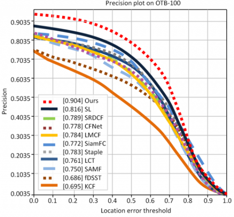
Ours |
0.608 |
0.904 |
Table 9. Result comparison of mean accuracy (TC-128)
|
TC128- Mean Success and Precision in % |
||
|
Tracker |
Success |
Precision |
|
KCF [33] |
0.418 |
0.588 |
|
Frag [34] |
0.408 |
0.538 |
|
VTD [35] |
0.407 |
0.527 |
|
MIL [36] |
0.393 |
0.539 |
|
OAB [37] |
0.389 |
0.526 |
|
SL [17] |
0.437 |
0.606 |
|
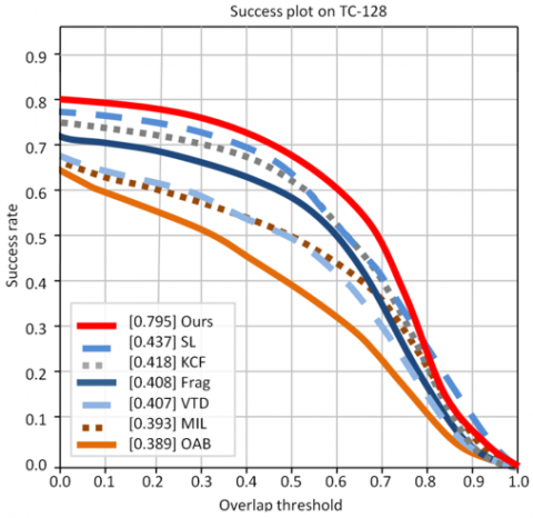
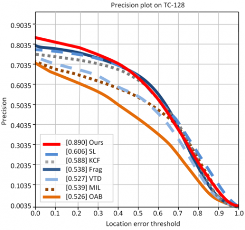
Ours |
0.795 |
0.890 |
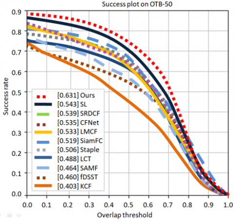
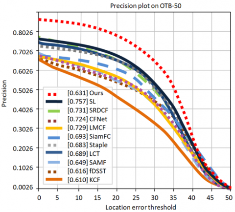
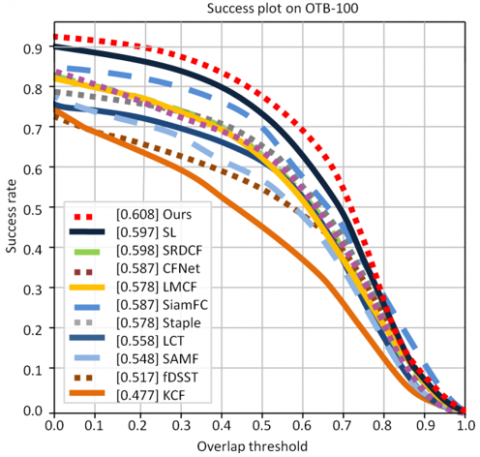
Figures 12 to 17 illustrate the performance evaluation plots for the three benchmark datasets. Specifically, Figures 12, 14, and 16 present the success plots for OTB-50, OTB-100, and TC-128 respectively, while Figures 13, 15, and 17 show the corresponding precision plots, providing a clear visual comparison of tracking accuracy and precision across these datasets.
Figure 12. Success Plot of OTB-50
Figure 13. Precision Plot of OTB-50
Figure 14. Success plot of OTB-100
Figure 15. Precision Plot of OTB-100
Figure 16. Success plot of TC-128
Figure 17. Precision plot of TC-128
Comparison of Evaluations Under 11 Attributes for OTB50, OTB100 and TempleColor128-Deformations (DEF), Illumination Variations (IV), Background Clutter (BC), In-Plane Rotations (IPR), Fast Motions (FM), Occlusions (OCC), Out of Plane Rotations (OPR), Motion Blurs (MB), Scale Variations (SV), Out of Views (OV) and Low Resolutions (LR).
In difficult scenarios with deformations, lighting variations, background clutter, in-plane rotations, fast motions, occlusions, out-of-plane rotations, motion blurs, scale variations, out-of-view instances, and low resolutions, the paper focuses on improving the tracking performance of Siamese Network and TensorFlow. When there are several peaks in the Siamese Network and TensorFlow response map, a more accurate detection network is used to pinpoint the object's position. Furthermore, the model retains accuracy in response to changes in the object's appearance. In addition, a high confidence template update technique is applied to avoid template contamination. The suggested system outperforms Siamese Network and TensorFlow in terms of tracking accuracy and success rates, according to an objective assessment using OTB and TempleColor sequences. Experiments on sample video sequences demonstrate better accuracy and resilience, especially in situations with varying lighting, fast motion, occlusion, and background clutter. Upcoming efforts will concentrate on improving the re-detection network and streamlining real-time performance to enable the engineering situations where Siamese Network based trackers may be used practically. Although it performs competitively on common tracking benchmarks, the suggested hybrid model that combines Siamese Networks and TensorFlow has some drawbacks. Specifically, the models performance may deteriorate in harsh settings like extended occlusion extreme target deformation or low light levels. Because of the limited information about appearance, these situations frequently result in tracking drift or loss of target identity. The use of multi-modal data adaptive appearance models or the integration of temporal attention mechanisms could all be investigated in future research. Adding transformer-based tracking modules or reinforcement learning could also help with occlusion recovery and adaptability to changing scenes.
[1] Ondrašovič, M., Tarábek, P. (2021). Siamese visual object tracking: A survey. IEEE Access, 9: 110149-110172. https://doi.org/10.1109/ACCESS.2021.3101988
[2] Lee, D.H. (2019). One-shot scale and angle estimation for fast visual object tracking. IEEE Access, 7: 55477-55484. https://doi.org/10.1109/ACCESS.2019.2913390
[3] Yan, B., Peng, H., Fu, J., Wang, D., Lu, H. (2021). Learning spatio-temporal transformer for visual tracking. In 2021 IEEE/CVF International Conference on Computer Vision (ICCV), Montreal, Canada, pp. 10448-10457. https://doi.org/10.1109/ICCV48922.2021.01028
[4] Husman, M.A., Albattah, W., Abidin, Z.Z., Mustafah, Y.M., Kadir, K., Habib, S., Islam, M., Khan, S. (2021). Unmanned aerial vehicles for crowd monitoring and analysis. Electronics, 10(23): 2974. https://doi.org/10.3390/electronics10232974
[5] Uke, N.J., Thool, R.C. (2014). Motion tracking system in video based on extensive feature set. The Imaging Science Journal, 62(2): 63-72. https://doi.org/10.1179/1743131X13Y.0000000052
[6] Zhong, W., Lu, H., Yang, M.H. (2012). Robust object tracking via sparsity-based collaborative model. In 2012 IEEE Conference on Computer Vision and Pattern Recognition (CVPR), Providence, USA, pp. 1838-1845. https://doi.org/10.1109/CVPR.2012.6247882
[7] Li, H., Wu, S., Huang, S., Lam, K.M., Xing, X. (2019). Deep motion-appearance convolutions for robust visual tracking. IEEE Access, 7: 180451-180466. https://doi.org/10.1109/ACCESS.2019.2958405
[8] Zheng, L., Tang, M., Wang, J. (2018). Learning robust gaussian process regression for visual tracking. In 2018 Twenty-Seventh International Joint Conference on Artificial Intelligence (IJCAI-18), Stockholm, Sweden, pp. 1219-1225. https://doi.org/10.24963/ijcai.2018/170
[9] Danelljan, M., Gool, L.V., Timofte, R. (2020). Probabilistic regression for visual tracking. In 2020 IEEE Conference on Computer Vision and Pattern Recognition (CVPR), Seattle, USA, pp. 7183-7192. https://doi.org/10.48550/arXiv.2003.12565
[10] Chen, K., Tao, W. (2018). Convolutional regression for visual tracking. IEEE TIP, 27(7): 3611-3620. https://doi.org/10.1109/TIP.2018.2819362
[11] Milan, A., Rezatofighi, S.H., Dick, A., Reid, I., Schindler, K. (2017). Online multi-target tracking using recurrent neural networks. In Proceedings of the AAAI Conference on Artificial Intelligence, 31(1): 4225-4232. https://doi.org/10.1609/aaai.v31i1.11194
[12] Yun, S., Choi, J., Yoo, Y., Yun, K., Choi, J.Y. (2018). Action-driven visual object tracking with deep reinforcement learning. IEEE Transactions on Neural Networks and Learning Systems, 29(6): 2239-2252. https://doi.org/10.1109/TNNLS.2018.2801826
[13] Henriques, J.F., Caseiro, R., Martins, P., Batista, J. (2014). High-speed tracking with kernelized correlation filters. IEEE Transactions on Pattern Analysis and Machine Intelligence, 37(3): 583-596. https://doi.org/10.1109/TPAMI.2014.2345390
[14] Zheng, L., Tang, M., Wang, J. (2018). Learning robust gaussian process regression for visual tracking. In 2018 Twenty-Seventh International Joint Conference on Artificial Intelligence (IJCAI-18), Stockholm, Sweden, pp. 1219-1225. https://doi.org/10.24963/ijcai.2018/170
[15] Li, X., Liu, Q., Fan, N., Zhou, Z., He, Z., Jing, X.Y. (2020). Dual-regression model for visual tracking. Neural Networks, 132: 364-374. https://doi.org/10.1016/j.neunet.2020.09.011
[16] Zhang, B., Zhang, X., Qi, J. (2015). Support vector regression learning based uncalibrated visual servoing control for 3D motion tracking. In 2015 34th Chinese Control Conference (CCC), Hangzhou, China, pp. 8208-8213. https://doi.org/10.1109/ChiCC.2015.7260942
[17] Zhang, J.W., Wang, H., Zhang, H.L., Wang, J.C., Miao, M.E., Wang, J.D. (2022). Tracking method of online target-aware via shrinkage loss. International Journal of Innovative Computing, Information and Control, 18(5): 1395-1411. https://doi.org/10.24507/ijicic.18.05.1395
[18] Danelljan, M., Hager, G., Shahbaz Khan, F., Felsberg, M. (2015). Learning spatially regularized correlation filters for visual tracking. In 2015 IEEE International Conference on Computer Vision (ICCV), Santiago, Chile, pp. 4310-4318. https://doi.org/10.1109/ICCV.2015.490
[19] Zheng, K., Zhang, Z., Qiu, C. (2022). A fast adaptive multi-scale kernel correlation filter tracker for rigid object. Sensors, 22(20): 7812. https://doi.org/10.3390/s22207812
[20] Yadav, S. (2021). Occlusion aware kernel correlation filter tracker using RGB-D. arXiv preprint arXiv:2105.12161. https://doi.org/10.48550/arXiv.2105.12161
[21] Maharani, D.A., Machbub, C., Yulianti, L., Rusmin, P.H. (2023). Deep features fusion for KCF-based moving object tracking. Journal of Big Data, 10(1): 136. https://doi.org/10.1186/s40537-023-00813-5
[22] Yang, J., Tang, W., Ding, Z. (2021). Long-term target tracking of UAVs based on kernelized correlation filter. Mathematics, 9(23): 3006. https://doi.org/10.3390/math9233006
[23] Oner, M.U., Kye-Jet, J.M.S., Lee, H.K., Sung, W.K. (2020). Studying the effect of mil pooling filters on mil tasks. arXiv preprint arXiv:2006.01561. https://arxiv.org/abs/2006.01561
[24] Xiong, D., Lu, H., Yu, Q., Xiao, J., Han, W., Zheng, Z. (2020). Parallel tracking and detection for long-term object tracking. International Journal of Advanced Robotic Systems, 17(2): 1729881420902577. https://doi.org/10.1177/1729881420902577
[25] Patil, R.R., Vaidya, O.S., Phade, G.M., Gandhe, S.T. (2020). Qualified scrutiny for real-time object tracking framework. International Journal on Emerging Technologies, 11(3): 313-319.
[26] Valmadre, J., Bertinetto, L., Henriques, J., Vedaldi, A., Torr, P.H. (2017). End-to-end representation learning for correlation filter based tracking. In Proceedings of the IEEE Conference on Computer Vision and Pattern Recognition, Honolulu, USA, pp. 2805-2813. https://doi.org/10.1109/CVPR.2017.298
[27] Wang, M., Liu, Y., Huang, Z. (2017). Large margin object tracking with circulant feature maps. In Proceedings of the IEEE Conference on Computer Vision and Pattern Recognition, Honolulu, USA, pp. 4021-4029. https://doi.org/10.1109/CVPR.2017.428
[28] Bertinetto, L., Valmadre, J., Henriques, J.F., Vedaldi, A., Torr, P.H. (2016). Fully-convolutional siamese networks for object tracking. In 2016 European Conference on Computer Vision Workshops (ECCV 2016 Workshops), Amsterdam, Netherlands, pp. 850-865. https://doi.org/10.1007/978-3-319-48881-3_56
[29] Bertinetto, L., Valmadre, J., Golodetz, S., Miksik, O., Torr, P.H. (2016). Staple: Complementary learners for real-time tracking. In 2016 IEEE Conference on Computer Vision and Pattern Recognition (CVPR), Las Vegas, USA, pp. 1401-1409. https://doi.org/10.1109/CVPR.2016.156
[30] Ma, C., Yang, X., Zhang, C., Yang, M.H. (2015). Long-term correlation tracking. In 2015 IEEE Conference on Computer Vision and Pattern Recognition (CVPR), Boston, USA, pp. 5388-5396. https://doi.org/10.1109/CVPR.2015.7299177
[31] Li, Y., Zhu, J. (2015). A scale adaptive kernel correlation filter tracker with feature integration. In 2016 European Conference on Computer Vision Workshops (ECCV 2016 Workshops), Amsterdam, the Netherlands, pp. 254-265. https://doi.org/10.1007/978-3-319-16181-5_18
[32] Danelljan, M., Häger, G., Khan, F., Felsberg, M. (2014). Accurate scale estimation for robust visual tracking. In 2014 British Machine Vision Conference (BMVC 2014), Nottingham, UK, pp. 1-12. https://doi.org/10.5244/C.28.65
[33] Henriques, J.F., Caseiro, R., Martins, P., Batista, J. (2014). High-speed tracking with kernelized correlation filters. TPAMI, 37(3): 583-596. https://doi.org/10.1109/TPAMI.2014.2345390
[34] Adam, A., Rivlin, E., Shimshoni, I. (2006). Robust fragments-based tracking using the integral histogram. In 2006 IEEE Computer Society Conference on Computer Vision and Pattern Recognition (CVPR), New York, USA, pp. 798-805. https://doi.org/10.1109/CVPR.2006.256
[35] Kwon, J., Lee, K.M. (2010). Visual tracking decomposition. In 2010 IEEE Computer Society Conference on Computer Vision and Pattern Recognition (CVPR), San Francisco, USA, pp. 1269-1276. https://doi.org/10.1109/CVPR.2010.5539821
[36] Babenko, B., Yang, M.H., Belongie, S. (2010). Robust object tracking with online multiple instance learning. TPAMI, 33(8): 1619-1632. https://doi.org/10.1109/TPAMI.2010.226
[37] Grabner, H., Grabner, M., Bischof, H. (2006). Real-time tracking via on-line boosting. BMVC Proceedings, 1(5): 6. https://doi.org/10.5244/C.20.6