Muthuraja Mani*![]() | Shanthi Natesan
| Shanthi Natesan![]() | Saravanan Thangavel
| Saravanan Thangavel![]() | Anguraju Krishnan
| Anguraju Krishnan![]()
© 2025 The authors. This article is published by IIETA and is licensed under the CC BY 4.0 license (http://creativecommons.org/licenses/by/4.0/).
OPEN ACCESS
In today's world, among 11 adults, one adult experiences diabetes mellitus and a complex illness known as diabetic foot ulcers (DFU). DFU needs to be treated well; otherwise, it may lead to amputation. The clinician performs the DFU treatment, where these treatments show remarkable restrictions, like costly diagnosis and lengthy care of DFU and treatment. Thus, there is a need for a novel decision-making technique. Constructing the dataset and collecting foot images from various patients are time-consuming processes. After the dataset acquisition, the skin conditions must be evaluated using computer vision algorithms. Here, novel learning techniques obtain the DFU features and the skin patches, which are healthy for understanding the difference in computer vision perspective. Further, the theoretical convolutional neural network architecture, CNN-DFUNet, is proposed to learn the feature representation to find the difference among the features and enhance the prediction accuracy. The CNN-DFUNet achieves 0.961 as the AUC score and is better than the conventional learning approaches. Furthermore, the proposed model is highly sensitive to detecting the presence of DFUs. Moreover, it is used for delivering the paradigm shift potentially among patients in diabetic foot care with less cost and reliable solutions in healthcare.
diabetic foot ulcer, machine learning, deep learning, convolutional network model, misclassification rate, feature representation, computer vision, prediction accuracy
Diabetes, also known as Diabetes Mellitus (DM), is a chronic condition resulting from high blood sugar levels, which can lead to serious health complications if not properly managed. It causes significant complications like kidney failure, cardiovascular diseases, lower limb amputation, and blindness that are frequently associated using Diabetic Foot Ulcers (DFU) [1]. In 2014, about 422 million individuals had DM, compared to 108 million people in 1980, based on the global report on diabetes. The global prevalence has crossed from 4.7% to 8.5% from 1980 to 2014 among adults 18 years of age [2]. Global DM prevalence is projected to reach 600 million individuals by 2035, according to estimates [3]. It is important to note that about 20% of people are from developed countries. The others are considered from developing countries because of the lack of awareness and the restricted facilities in healthcare [4]. A diabetic patient has a chance of about 15% to 25% developing DFU eventually, and the lower limb amputation may occur if the proper care is not taken [5]. More than 1 million patients have DM lose their leg part every year because they fail to identify it and treat the DFU properly [6]. A ‘high risk’ foot requires a periodic check-up with the doctors for the diabetic patient with continuous medication, which is costly, and hygienic personal care is needed to protect from additional problems mentioned before. Hereafter, an extensive burden will be caused, burdening the patient's family and the patient, particularly in developing countries. Here, the expense of treatment for the disease is costly and equal to 5.7 years of annual income [7].
The determination of DFU consists of different vital works in the present clinical practices and early diagnosis, which keep track of enhancement, and the count of lengthy tasks is considered in the management and treatment of DFU in every specific case [8]. They are (i) the evaluation of the patient's medical history needs to be considered, (ii) a specialist of the diabetic foot and the wound is examined the DFU thoroughly, (iii) the extra tests such as MRI, CT scans, and X-ray are required for helping to help plan the treatment [9]. Based on every scenario, the DFU patients have swollen legs, even though it is painful and itchy. The DFU appearance visually and the skin around the wound is based on the different phases, like callus formation, redness, numerous types of tissues such as slough, granulation, scaly skin, bleeding, and blisters [10-12]. Generally, uncertain outer boundaries and irregular structures are there in DFU. Evaluating ulcers with computer vision algorithms depends on correctly assessing the visually considered signs as texture features and colour descriptors. However, all these methods fail to provide a substantial outcome for predicting cancer in the earlier stage. Thus, some complexities are not addressed by the existing works. They are: (i) collection requires more time and the DFU images are labelled by experts, (ii) the high inter-class similarity among the abnormal classes as DFU and regular classes as healthy skin, and the intra-class variations that are based on the DFU classification [13], the ethnicity of the patient, and the lighting conditions. Research in foot ulcer prediction using deep learning has made significant strides, particularly for diabetic patients, yet several critical gaps and limitations remain. Addressing these issues is essential to improving model performance, generalizability, and clinical relevance. One major limitation is the scarcity and imbalance in existing datasets. Most available datasets for foot ulcer prediction are small, with a disproportionate number of images representing advanced-stage ulcers compared to early-stage cases. This imbalance hinders a model's ability to generalize and accurately detect the early signs of foot ulcers. To enhance generalizability, there is a need for larger, well-annotated, and diverse datasets that include various stages of foot ulcers across different demographics, including skin tones and patient age groups. Another challenge is the interpretability of DL techniques, specifically CNNs, which are often perceived as "black boxes." Clinicians and medical experts require models that provide transparent and interpretable predictions to confidently integrate them into clinical workflows. Without interpretability, there may be hesitation to trust or adopt these AI systems in real-world settings. Early detection of foot ulcers remains an ongoing challenge. While current models perform well in predicting advanced-stage ulcers, they often struggle to identify early-stage ulcers where signs may be more subtle. Models trained on small, imbalanced datasets are prone to overfitting, reducing their effectiveness when applied to new, unseen data. Therefore, improving model robustness and preventing overfitting are key areas where progress is needed, particularly when training data is limited. Addressing these gaps can give rise to more accurate, interpretable, and clinically viable models for foot ulcer prediction. Techniques like multimodal learning, real-time monitoring, and explainable AI have the potential to enhance the applicability and effectiveness of these models in healthcare settings. Additionally, comparing the proposed model with existing methods such as LBP, LeNet, AlexNet, GoogleNet, HOG+LBP, and color descriptors is important for benchmarking performance. Improving the model's ability to detect early-stage ulcers would enable more effective preventive interventions, which is crucial for patient outcomes. Nonetheless, the proposed model shows promising results in terms of accuracy, recall, F1-score, and precision, offering a groundwork for future enhancements in this area.
Thus, the proposed model intends to address these issues with the proper clinical findings in the earlier stage. The computer vision approaches are proposed to differentiate the DFU with deep learning and conventional machine learning techniques from healthy skin [14, 15]. The proposed system shows some major contributions as listed below:
1) Here, a novel computerized telemedicine system is presented to address the issues in DFU. The input dataset consists of 397-foot image samples, where 292 samples show DFU and 105 images of a healthy foot.
2) Subsequently, a novel learning approach is employed to learn and extract the features from the patches of healthy skin and the DFU. With the boom of DL, CNNs are used to develop the fully automated technique for classifying the DFU skin over the regular skin.
3) The proposed CNN-DFUNet is developed with fine-tuned input data and works more effectively than the modern CNN. It requires the actual data to generate the exact outcomes, yet in the convolutional blocks parallel with the larger filter size of CNN-DFUNet, which can create better results on the dataset.
The work is structured as follows: Section 2 offers a comprehensive evaluation of existing techniques and discusses the benefits and drawbacks related to the model. Section 3 provides an elaborate discussion on the proposed CNN-DFCNet model. The numerical results are provided in Section 4, followed by the research summary in Section 5.
The communication technologies and the proliferation of information represent both the chances and difficulties of the new age medical systems development. The number of e-health systems is available in developing levels, like (i) the present healthcare systems are improved, and the expense of medical facilities are decreased, (ii) a level of medical facilities is improved such as that patients' remote assessment are often suits with the less expert medical professionals to the chronic disease [9]. Doctors and researchers have designed critical telemedicine systems over the years to monitor diabetes [16, 17]. Moreover, some intelligent systems are proposed for the pathologies of the diabetic foot that need to be classified into automated and non-automated telemedicine systems. With the sudden development in mobile telecommunications, remote communication has standalone devices such as laptops, the Internet, and smartphones. In today's world, small smart devices, like pocket-sized having enhanced mobile operating systems, have the personal computer's abilities. It captures high-resolution images, video, and audio communication and has an improved mobile Internet, such as 4G. The general telemedicine systems in the non-automatic criteria depend on the devices that are almost needed to arrange for the patients' assessments in the remote location, such as (i) three-dimensional wound imaging (3D), (ii) video conferencing, (iii) optical scanner, and (iv) digital photography [18]. Moreover, specialized medical professionals are still needed to complete the patients' assessment. There is an urgent requirement for intelligent systems that can detect the pathologies of DFU automatically and remotely, even though the systems give guaranteed outcomes.
The automatic telemedicine systems for DFU usage are still in inception. It is important to note that the intelligent telemedicine system was designed by Hermans [19] in 2015 to detect the complications of diabetic food by having infrared thermal images, reconstruction of 3D surface, and spectral imaging. Moreover, there is a need for different costly devices, and special training is required for using the devices to implement this system. Foltynski et al. [20] use the image capture box to obtain the image features and evaluate the DFU's area with the help of cascaded two-staged related classification such as Support Vector Machine. The proposed system uses the super-pixel approach to segment and extracts the feature number for performing two-staged categorization. Even though the system reports the guaranteed outcome, this is not validated on the larger dataset. In addition, data collection is not possible through the image capture box. There is a requirement to contact the box surface and the patient's foot, which is not permitted in the healthcare setting due to infection control. Chen et al. [21] developed the DFUs' segmentation, and the skin is surrounded by the whole foot image in other remarkable areas.
In addition, the manual or image processing techniques or the engineered features are related to the computer methodologies established to classify the tissue and the skin lesion, like the wound is segmented. The process of extracting the different features, like the colour descriptors and the texture descriptors, on the less delineated patches of wound images, is used to perform the classification task with the help of conventional machine learning. It is used for classifying skin patches as abnormal and normal classes using machine learning algorithms [22-25]. The skin colour and the lighting conditions affect the hand-crafted features in multiple computer vision systems based on the patient's ethnicity. Generally, all skin lesions are virtually related to the ulcer, which is termed a wound. The ulcer and the injury are concerned differently in the medical perspective produced using the external issue. On the other hand, internal problems cause an ulcer. In addition, the skin lesion has a different appearance from ulcer and wound. The scenario is based on the body works like physiology, aetiology and pathology [25]. Moreover, DFU alone is concerned in the current research for determining how these are varied from the physically regular skin at the place of appearance.
In recent years, there have been sudden enhancements in the computer vision area mainly to critical and challenging problems such as the images being understood with various domains like medical, spectral, detection of an object, and face, label classification and multi-class classification [26]. The machine learning algorithms and traditional computer vision are significantly fewer capabilities for processing the wide range of image data, which gives the data representation various levels of abstraction and requires more tuning in manual way for every input image. A recent machine learning algorithm called deep convolutional networks rises as the fundamental approach for solving the types of problems in computer vision [27]. It transforms the simple representation of features into a more enhanced abstract model for categorization. Simple non-linear modules are employed to acquire the different levels of representation approaches using DCN. The image samples are used as input and begin to understand the features like position from the array of pixel values and the edges at a particular direction by the deep convolutional networks. The combination of the edges at a greater level needs more vital abstract features, like the components of the required object. In the last stage, the components are associated with forming the final object [28]. One of the general forms of ML is supervised learning. It is necessary to train the system's classification tasks from the broad group of images distinctly labelled for every category. It is impossible to detect the needed class without training using the most incredible score of all the types [29]. During the training phase, the machine processes the various images to generate the scores vector output for every image for all classes. Thus, the errors are evaluated related to output scores rather than the predicted score until every class's reliable score is attained. After the training, a set of images is validated to fine-tune the networks' hyper-parameters like weights, pooling layer counts and the convolutional layers. Finally, the system's performance is checked by testing the system and real-world test data with no predicted result [30]. Table 1 depicts the comparison of various existing approaches.
Table 1. Summary of DFU prediction using various deep and machine learning approaches
|
S. No |
Author |
Wound Type |
ES |
Total Patients |
ES Parameters |
Duration |
Outcomes |
|
1 |
[21] |
DFU |
HPVC |
41 |
100 $\mu s$ and 50V |
12 weeks with 8h |
The healing rate is higher compared to other approaches |
|
2 |
[22] |
Chronic diabetic ulcers (CDU) |
Heat+ES+local dry heating |
21 |
30Hz, 20mA and 250 $\mu s$ |
35 min with 4 weeks |
Increased healing rate with local heat |
|
3 |
[23] |
CDU and DFU |
LIDS |
48 |
1.5$\mu A$ |
60 min with 8 weeks |
Increased healing rate |
|
4 |
[24] |
Open diabetic ulcers |
HPVC |
30 |
100$\mu s$ and 140V and 55Hz |
45 min+4 weeks |
Enhanced healing rate |
|
5 |
[25] |
Chronic leg ulcer (CLU) |
Asymmetric biphasic pulsed current |
80 |
-- |
Ulcer healed |
The increased healing rate is 65% |
|
6 |
[26] |
DFU |
HPVC |
28 |
150V, 100$\mu s$ and 100Hz |
50 min |
The wound size is reduced in the initial phase |
|
7 |
[27] |
Stage IV decubitus ulcer |
ES+global heat ES+local+heat |
30 |
30Hz and 20mA |
30 min |
The healing rate is higher with global heat |
|
8 |
[28] |
CLU |
HPVC |
15 |
100V, 50$\mu s$ and 105Hz |
50 min |
45% healing rate is seen |
|
9 |
[29] |
CLU |
FIRMS |
35 |
100Hz, 10-40$\mu s$ and 100V |
45 min and 3 weeks |
Improved healing rate |
|
10 |
[30] |
DU |
Placebo vs ENS |
65 |
-- |
50-60 min and 12 weeks |
Reduced pain and enhanced healing rate |
CNN-DFUNet may feature a custom architecture specifically optimized for foot ulcer detection, designed to capture the unique characteristics of ulcers, such as texture, color variations, and irregular shapes. This specialized design likely enhances feature extraction compared to general-purpose networks. To determine whether CNN-DFUNet’s AUC score of 0.961 signifies a statistically significant improvement over other methods, statistical tests like the DeLong test for comparing AUCs, McNemar’s test, or a paired t-test (for accuracy, sensitivity, etc.) could be employed. Additionally, calculating confidence intervals for AUC scores and other performance metrics would clarify whether the observed improvements are statistically significant or likely due to chance. Applying cross-validation techniques (e.g., k-fold) and comparing the average results across folds would further help assess if CNN-DFUNet consistently outperforms alternative models. Its superior performance can be attributed to its customized architecture, multi-scale feature extraction, ability to handle data imbalances, and efficient learning methods. To confirm that this improvement is statistically significant, proper statistical testing and cross-validation should be conducted.
This section provides a broader assessment of the proposed model. Here, a novel CNN-based DFUNet is proposed to analyze diabetic foot ulcer prediction and classify diabetic ulcer stage (classes). Here, some essential pre-processing steps are done before performing classification. The performance of the anticipated model is measured using metrics like sensitivity, accuracy, specificity, precision, F-measure, SE and CI.
3.1 Dataset
The dataset of DFUs standardized colour images requires being collected from different patients to train the other deep learning models. The extensive dataset, having 292 patients' foot images of the DFU, has been used across the prior five years in the Lancashire Teaching Hospitals to ethically obtain approval from the appropriate patients and bodies that provide written consent of information. In addition, about 105 healthy foot images are gathered to get more scenarios for the typical healthy classes. The NHS Research Ethics Committee provides approval for using the images for the study. Nikon D3300 is used to capture the DFU images. The images show a complete foot whenever needed, with a distance of around 30 to 40cm to the plane of an ulcer having a parallel orientation. The flash is the first light source that can be eliminated, rather than using suitable room lights to get reliable colours in the images. The Nikon AF-S DX Micro NIKKOR 40mm f/2.8G lens is utilized to ensure close-up focus and eliminate the blurriness from the close-up distance in the images. Another test case is added in the proposed system to capture with the help of the FootSnap application with an iPad to show the meaningful algorithms across the heterogeneous capturing setup. This heterogeneous test case comprises 32 regular and 20 abnormal skin patches.
3.2 Image labelling
Zhou et al. [30] provide a suitable annotator for every full image of the foot that has ulcers and the Region of Interest (ROI) delineated by medical experts in the crucial area above the ulcer, with both abnormal and normal skin tissues.
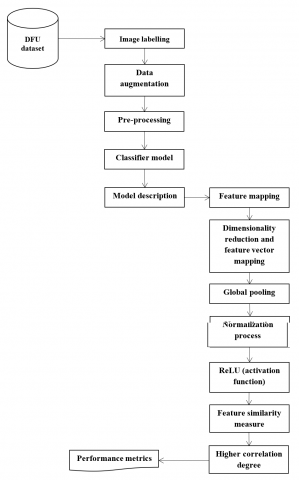
Figure 1. Flow of the anticipated model
Figure 1 illustrates the workflow of the proposed model. The medical professionals outline the ground truth labels in infected skin patches and normal skin patches from the area of the ROI. The ground truth of the abnormality type is labelled and exported for every delineated abnormal area to the Extensible Markup Language (XML) file. The experts gathered both the patch classes from the region of ROI in the group of ground truth patches, which helps have a more meaningful categorization of the patches than involving the complete foot as the area. There are about 292 ROI, such as only for ulcers; foot images for the annotation of 397-foot images having both the non-ulcer and ulcer with 1679 skin patches, have the 1038 abnormal class and the 641 normal classes from these annotations. Lastly, the dataset is divided into 84 patches for validation, 1423 for the training, and 172 for testing.
3.3 Data augmentation
The deep networks need more training image data due to the many parameters. The learning algorithms assign the weights with the convolutional layers, which can be tuned. Moreover, data augmentation enhances deep learning techniques. Different image processing approaches, such as flipping, rotation, and enhancement of contrast, are combined with the help of random scaling and the various colour spaces for data augmentation. Angles of 90° and 180° rotate the image, and 270° is used for further rotation. Thus, the three flipping methods, vertical flip, horizontal flip, and horizontal and vertical flip, are needed to serve on the original patches. Four colour spaces are required to augment data like NTSC, HSV, $L * a * b$, and YCbCr. There are three functions in contrast enhancement. The two cropped patches having the random orientation and the random offset are produced in the proposed system from the skin patches in the original dataset. The amount of training and validation patches is increased by fifteen times, that is, 1260 patches for validation and 21,345 patches for training with these approaches.
3.4 Pre-processing
There is a necessity for pre-processing on these patches since many training data augments are obtained. The zero-centre approach is utilized to pre-process these attained patches, and then the normalization is done for each pixel.
3.5 Classifier model
The proposed CNN-DFU model is a lightweight model that reduces complexity and enhances processing speed. The model intends to reduce the computational complexity and processing speed. The novelty of the work relies on the layer description and the changes done between the standard feature extraction layer of CNN and the fully connected layer. The features are analyzed, and the approximation with the extracted linear features is derived.
3.6 Model description
Assume $\chi$ is the set of $N$ images where the feature maps are obtained from the $i^{\text {th }}$ image with the feature extraction block. There is no constraint with the architectural model adopted for the feature extraction procedure. Consider $L$ as the number of layers (lightweight) where the features are extracted. Here, $X_{i j} \in \mathbb{R}^{N_f}$ is adopted for the extracted feature vector for the $i^{t h}$ image of $\chi$, and $N_f$ is the convolutional layers' channel (features extracted). The length of the feature maps describes several feature vectors, which are available across the intermediate layers. The feature vector count defines the feature map size and is available over the extracted feature. For instance, when the $20 * 20$ feature maps are extracted, the vectors are provided for different quantization processes. The factor $N_i$ extracts several feature vectors from the available $i^{\text {th }}$ mage. The image is specified with the set of $N_i$ feature vectors $x_{i j} \in \mathbb{R}^{N_F}\left(j=1, \ldots, N_i\right)$ extracted with the trained convolutional feature extractor. The intermediate layers are compiled using the histogram generated for every image after feature vector quantization. The prevailing global pooling approaches are fused with the feature vectors or used for pooling the spatial information for feature representation. The proposed model decouples the extracted feature representation size based on dimensionality and feature vectors. It facilitates independently controlling the feature representation size and allows the reduction of layer parameters required by the fully connected layers.
Input layer: It also helps in handling images of various sizes. Similarly, two diverse layers are utilized to examine the extracted features: 1) one layer measures the input feature vector similarity and measures the input vectors, and 2) accumulation layers execute the histogram representation by integrating the feature vectors (quantized). Thus, the layers form the pooling structure used for extracting the representation, which is fed as an input to the successive classifier. The differential similarity function is adopted to measure the feature vectors' similarity issues. The feature formulation of the anticipated model relies on the kernel-based radial basis function, which is used as a similarity metric. Thus, the RBF neurons are included in the preliminary layers, and the output of $k^{\text {th }}$ neuron $[\emptyset(x)]_k$ is expressed in Eq. (1):
$[\emptyset(x)]_k=\exp \left(-\left.\left\|x-v_k\right\|\right|_2 / \sigma_k\right) \in \mathbb{R}$ (1)
Here, $v_k$ refers to the number of features and feature representation size. Where $x$ specifies the feature vector, $v_k$ is the output of the k -th neuron, and $\sigma_k$ is the scaling factor used to adjust the Gaussian function in RBF neurons over the intermediate layers. Then, $l^1$ scaling is used for feature formulation and normalization is applied over the neurons. The output from the RBF neuron is represented in Eq. (2):
$[\emptyset(x)]_k=\frac{\exp \left(-\left|\left|x-v_k\right|\right|_2 / \sigma_k\right)}{\sum_{m=1}^{N_k} \exp \left(-\left|\left|x-v_m\right|\right|_2 / \sigma_m\right)}$ (2)
It can be efficiently understood by the feature vector quantization and normalizing of the higher similarity feature vectors. The normalization process is adapted to the layers of the anticipated model to ensure the distribution shift and enhance the scale invariance. The enhanced scale invariance of the expected model is shown in Figure 1. The final image representation is extracted based on the RBF neuron response of every vector, and it is fed to the intermediate layers, and it is expressed in Eq. (3):
$s_i=\frac{1}{N_i} \sum_{j=1}^{N_i} \emptyset\left(x_{i j}\right) \in \mathbb{R}^{N_k}$ (3)
Here, $\emptyset(x)=\left([\emptyset(x)]_1, \ldots,[\emptyset(x)]_{N_k}\right)^T \in R^{N_k}$ specifies the RGF vector output, and $s_i$ specifies the histogram, which is expressed based on the distribution of RBF neurons and determines the visual content of every sample image. The $s_i$ vectors possess an $l^1$ normalization unit. It is provided to the fully connected layers-the extracted features from the histogram and projects the feature vector distribution with the elimination of spatial information. The spatial information is provided to the extracted feature representation, which is like of matching technique. The images are segmented to the number of regions, and individual histograms are acquired from one another. The histograms are integrated to produce the resultant representation. The representation is provided as $N_K N_S$, where $N_S$ specifies the total spatial regions. The classifier model needs to infer the image class after hauling out the histogram representation and the model with loss function (differential) is utilized for analysis.
Hidden layer: The multi-layer perceptron with the hidden layer is specific to the anticipated model. The quantity of hidden neurons is specified as $N_H$, while the output neuron is utilized for every class that leads to output layer $N_c$ (classification problem for various courses). Nc specifies the total hidden neurons, the regression is performed, and the neuron's output is set as $N_c=1$.
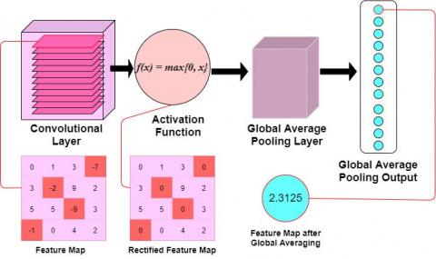
Activation layer: The ReLU activation function with hyper-parameters (default) is utilized for hidden layers. With the ReLU, the obtained histograms enhance the network convergence velocity over the various activation functions. The softmax layer is employed for the classification of output layer, while regression does not employ any activation function. The classification process used cross-entropy loss function for network training, whereas regression used squared loss function. The dropout is set as $p=0.5$ is utilized for the hidden layer, and gradient descent is used for learning the attributes, and it is shown in Eq. (4):
$\begin{aligned} & \Delta\left(W_{M L P}, V, \sigma, W_{c o n v}\right) \\ & =-\left(\eta_{M L P} \frac{\partial L}{\partial W_{M L P}}, \eta v \frac{\partial L}{\partial V}, \eta_\sigma \frac{\partial L}{\partial \sigma}, \eta_{c o n v} \frac{\partial L}{\partial W_{c o n v}}\right)\end{aligned}$ (4)
Here, the symbol $L$ is utilized to specify the loss function, $\sigma$ sets the scaling factors $\left(\sigma=\left(\sigma_1, \ldots, \sigma_{N_K}\right)\right)$, and $V=$ ( $v_1, \ldots, v_{N_K}$ ) identifies the RBF neurons (centroid). The classifier and feature parameters are expressed as $W_{M L P}$ and $W_{\text {conv }}$, respectively. The learning rate of the parameters is specified as $\eta_{M L P}, \eta v, \eta_{\text {sigma }}$, and $\eta_{\text {conv }}$. The adam optimizer is used to perform optimization, and the derivations from the intermediate layers are derived analytically using supplementary materials. The convolutional feature extraction is initialized randomly or pre-trained. In MLP, $k$ - means is initialized, and the vectors $S=\left\{x_{i j} \mid i=1, \ldots, N, j=\right.$ $\left.1, \ldots, N_i\right\}$ are clustered to $N_K$ clusters and centroids $V K \in$ $\mathbb{R}^{N_F}\left(k=1, \ldots, N_K\right)$ are utilized for initializing the neurons centroid. The process is adopted for learning purposes, applied for centre initialization and optimized to fulfil the objective. The scaling factor is set as 0.1. At last, the random initialization process is utilized for MLP parameter initialization.
The critical concept that relies on linear feature pooling is to substitute the higher non-linear similarity evaluation that performs computation with pairwise distance and transforms the RBF kernel similarity, i.e., linear operator. The non-linear exponential operator and scaling factor adopted in Eq. (1) are eliminated and attain the similarity function.
$[\emptyset(x)]_k=-\left.\left\|x-v_k\right\|\right|_2 \in \mathbb{R}$ (5)
The above Eq. (5) can also be developed with the squared distance among the feature vectors.
$[\emptyset(x)]_k=-\left|\left|x-v_k\right|\right|_2^2=2 x^T v_k-||x||_2^2-\left|\left|v_k\right|\right|_2^2$ (6)
Thus, the similarities among the feature vectors are specified as the inner product among the vectors after subtracting $l^2$ normalization. After the training, the normalization factor is set constant, i.e. $\left\|v_k\right\|_2^2=c_k$. Consider that the feature vector normalization is constant, and $\left|\left|v_k\right|\right|_2^2=$ $c_f$ is reduced to $[\emptyset(x)]_k=2 x^T v_k-c$, where $c=c_k+c_f$ is a constant (fixed). Thus, with the elimination of additive factor " $c$ ", the similarity function is given by Eq. (7):
$[\emptyset(x)]_k=C^{S T} v_k$ (7)
The above Eq. (7) represents the cosine similarity $\left(\left(x^T v_k /||x||_2| | v_k| |_2\right)\right)$ with unit length representation. Moreover, the unit length ranges from $-\infty$ to $\infty$ while cosine similarity ranges between -1 and 1. To avoid normalization during network deployment, the absolute operator fulfills the similarity metrics and leads to similarity metrics for linear feature analysis.
$[\bar{\bar{\phi}}(x)]_k=\left|x^T v_k\right| \in \mathbb{R}$ (8)
where, |$.$| specifies the absolute value operator. The similarity value specifies a higher correlation degree with (+ $ve$ and - $v e)$ vectors, while values nearer to 0 specify the no correlation factor. The anticipated similarity metrics eliminate the correlation sign. It may not harm the model accuracy, as the degree of correlation among the vectors, i.e., essential information. Moreover, the feature vectors are provided to the similarity metrics, and the gradients are back-propagated to the related layers with the elimination of the correlation sign. The quantization used over the regular pooling operations is evaluated with Eq. (9):
$[\bar{\bar{\emptyset}}(x)]_k=\frac{\left|x^T v_k\right|}{\sum_{m=1}^{N_k}\left|x^T v_m\right|}$ (9)
Then, the histogram representation is hauled out using the membership vectors. The gradient descent is utilized for parameter learning, and the derivatives are attained analytically. Since Euclidean clustering is not employed during the similarity assessment between the feature vectors, the linear pooling is not enhanced by k-means initialization. The pooling layer is provided sequenced, and the average pooling layer is set with proper strides and a pooling window (Figure 2).
Figure 2. Internal representation of the network model
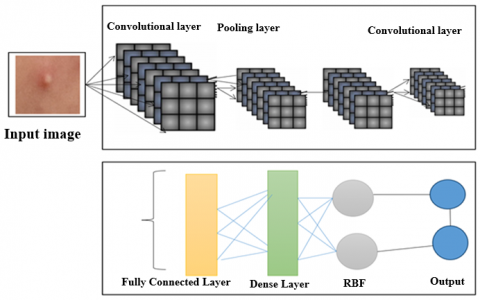
Figure 3. CNN-DFUNet model
Convolutional layers: The similarity evaluation is executed as the absolute value operator in the convolutional layer. Thus, $N_K$ is the filter size $\left(1 * 1 * N_F\right)$, and $N_f$ specifies the filter count. Moreover, with the experimentation, it is noted that the skipping normalization does not affect the performance of the pooling. At last, average pooling with stride and window length equal to the extracted feature length maps are utilized to extract the input sample representation as a feature size map $1 * 1 * N_k$. As the independent histogram is hauled out, the spatial segmentation needs to alter the window length, i.e. diminishing the window length is equal to the spatial segmentation (i.e., level=1). The segmentation process provides the spatial regions. However, it does not diminish the model's learning ability and reduces the overfitting risk. The architecture adopted for executing the linear variants is similar to the network, i.e., $1 * 1$ convolutions to diminish the extracted features. The network model provides a primitive way of removing the feature representation and gives successive insights (Figure 3).
The feature extraction model is competent in decoupling the feature representation from the extracted feature count and its dimensionality, allowing the network model. The CNN model needs $O\left(N_i N_F N_H+C_L\right)$ parameters for the fully connected layers, the pooling layer needs $O\left(N_F N_H+C_L\right)$, and the linear features require $O\left(N_S N_K N_F+N_S N_K N_H+C_L\right)$. The parameters are diminished to $O\left(N_K N_F+N_S N_K N_H+C_L\right)$. The cost of evaluating the network process is $O\left(N_i N_F N_H+\right.$ $\left.C_L\right), O\left(N_i N_F+N_F N_H+C_L\right)$ for global mapping and $O\left(N_i N_K N_F+N_S N_K N_H+C_L\right)$ for feature mapping. The cost to assess the similarity among the feature vectors is the same for the linear feature. The distance among the vectors is evaluated with the product evaluation, i.e., $\|x-y\|_2^2=x^T x+y^T y-$ $2 x^T y$ for two diverse features vectors $x$. The obtained feature count is based on the input image dimension. Therefore, the complexity is handled by the global mapping and linear feature analysis with the suitable input image.
The dataset of DFU is divided into 5% validation, 10% testing sets, and 85% training, and the 5-fold cross-validation approach is adopted in the proposed system. Henceforth, the proposed method has the CNN-DFUNet architecture for validation, training, and testing set, and about 84 patches comprising 52 abnormal cases, 1423 patches comprising 882 irregular cases, and 172 patches, such as 104 irregular cases from the 397 exact image samples of the foot. The earlier proposed system uses CNNs and CML models to perform the classification task. Table 1 depicts the performance of various metrics like specificity, sensitivity, accuracy, precision, AUC, and F-measure. In healthcare imaging, specificity and sensitivity are the more reliable metrics to measure classifier efficiency.
$Sensitvity =\frac{T P}{T P+F N}$ (10)
$Specificity =\frac{T N}{F P+T N}$ (11)
$Precision =\frac{T P}{T P+F P}$ (12)
$Accuracy =\frac{T P+F N}{T P+T N+F P+F N}$ (13)
$F-measure$=$\frac{2 * T P}{2 * T P+F P+F N}$ (14)
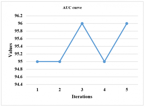
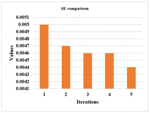
The performance measures for different CNN-DFUNet variants are reported in Table 2, having the various parameters described in the CNN-DFUNet architecture in the previous step. There is no more gap in the efficiencies of all the appraoches. Yet, CNN-DFUNet Iteration 5 is made better in each evaluation metric without precision; here, CNN-DFUNet iteration 1 performed well. The earlier hypothesis is correct, like increased filter size in the parallel convolution layers needed to enhance the CNN-DFUNet efficiency. Moreover, CNN-DFUNet iteration 5 utilizes larger filter sizes than the other variants in the previous two similar convolutional layers, creating good outcomes. Henceforth, the CNN-DFUNet is proposed with the good results that CNN-DFUNet obtains for comparing the deep learning models and other conventional machine learning performances. Table 3 compares various performance metrics. The work is performed for successive iterations, i.e., iteration 1 to iteration 5. The sensitivity ranges from 92% to 95% from iteration 1 to iteration 5. The specificity ranges from 91% to 95% from iteration 1 to iteration 5. The precision ranges from 94% to 91% from iteration 1 to iteration 5. The accuracy ranges from 91% to 95% from iteration 1 to iteration 5 (Figure 4). The F-measure ranges from 93% to 93% from iteration 1 to iteration 5. AUC ranges from 95% to 96% from iteration 1 to iteration 5 (Figure 5). The SE ranges from 0.0050 to 0.0040 (Figure 6), and the CI ranges from 0.94 to 0.96 (Figure 7).
Table 2. Performance evaluation comparison
|
Iterations |
Sensitivity |
Specificity |
Precision |
Accuracy |
F-Measure |
AUC |
SE |
CI |
|
1 |
0.92 ± 0.030 |
0.91 ± 0.053 |
0.94 ± 0.039 |
0.91 ± 0.03 |
0.93 ± 0.03 |
0.95 |
0.0050 |
0.94-0.96 |
|
2 |
0.92 ± 0.023 |
0.90 ± 0.032 |
0.94 ± 0.02 |
0.91 ± 0.04 |
0.93 ± 0.02 |
0.95 |
0.0047 |
0.94-0.96 |
|
3 |
0.92 ± 0.028 |
0.90 ± 0.028 |
0.94 ± 0.025 |
0.92 ± 0.03 |
0.93 ± 0.02 |
0.96 |
0.0046 |
0.95-0.96 |
|
4 |
0.92 ± 0.025 |
0.90 ± 0.063 |
0.93 ± 0.03 |
0.91 ± 0.04 |
0.93 ± 0.01 |
0.95 |
0.0046 |
0.94-0.96 |
|
5 |
0.95 ± 0.025 |
0.91 ± 0.030 |
0.94 ± 0.03 |
0.95 ± 0.02 |
0.93 ± 0.02 |
0.96 |
0.0044 |
0.95-0.96 |
Table 3. Comparison of proposed vs existing approaches
|
Existing Vs. Proposed |
Sensitivity |
Specificity |
Precision |
Accuracy |
F-Measure |
AUC |
SE |
CI |
|
LBP |
91 |
76 |
87 |
86 |
89 |
93 |
0.0062 |
0.92 |
|
HOG+LBP |
89 |
84 |
90 |
86 |
89 |
93 |
0.0061 |
0.91 |
|
HOG+LBP+Color descriptors |
90 |
84 |
90 |
88 |
90 |
94 |
0.0055 |
0.93 |
|
LeNet |
91 |
81 |
87 |
87 |
89 |
92 |
0.0050 |
0.94 |
|
AlexNet |
89 |
88 |
93 |
89 |
91 |
95 |
0.0051 |
0.94 |
|
GoogLeNet |
90 |
91 |
94 |
90 |
92 |
96 |
0.0046 |
0.95 |
|
DFUNet |
93 |
91 |
94 |
92 |
93 |
96 |
0.0045 |
0.95 |
|
Proposed |
95 |
93 |
94 |
95 |
95 |
97 |
0.0030 |
0.97 |
Figure 4. Performance analysis
Figure 5. AUC plotting
Figure 6. SE evaluation for successive iterations
Figure 7. CI evaluation for subsequent iterations
Three diverse conventional machine learning (ML) approaches and three modern CNN approaches are considered for classification purposes. In the traditional ML approaches, HOG, LBP, and colour descriptors are used as feature vectors and trained with some optimization approach to perform classification. Some modern CNNs include GoogLeNet, AlexNet, and LeNet, which are considered for analysis with the proposed CNN-DFUNet model. Every classifier is efficient in its way and works effectually; however, the sensitivity of those classifiers is substantially lower than the anticipated model. Similarly, the proposed CNN-DFUNet model is also efficient in the case of specificity, with the results ranging from 0.76 to 0.93. The CNN performs better than the most conventional ML features using a more significant margin. In many scenarios, all the CNN architectures obtain more excellent outcomes than ML. The best performers are CNN-DFUNet and GoogLeNet to evaluate the different metrics between the classifiers. The demonstration of the receiver operating characteristic curve for all the models is made.
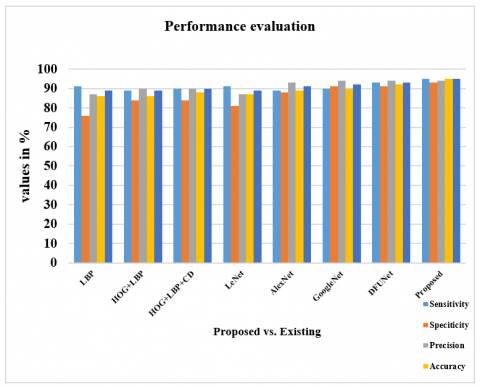
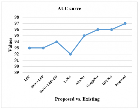
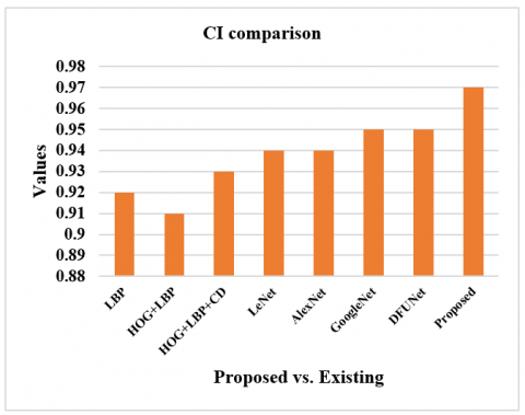
Table 3 compares the anticipated model with the existing approaches like LBP, HOG+LBP, HOG+LBP+color descriptors, LeNet, AlexNet, GoogLeNet, and DFUNet. The sensitivity of the proposed model is 95% which is 4%, 6%, 5%, 4%, 6%, 5% and 2% more than the existing models. The specificity of the proposed model is 93% which is 17%, 9%, 9%, 12%, 5%, 2% and 2% more than the existing models. The precision of the anticipated model is 94% which is 7%, 4%, 4%, 7%, and 1% higher than other approaches and equal to GoogleNet and DFUNet, respectively. The accuracy of the anticipated model is 95% which is 9%, 9%, 7%, 8%, 6%, 5% and 3% more than the existing models, and all of these metrics are shown in Figure 8. The F-measure of the anticipated model is 95% which is 6%, 6%, 5%, 6%, 4%, 3% and 2% more than the existing models. The AUC of the anticipated model is 97% which is 4%, 4%, 3%, 5%, 2%, 1% and 1% more than the existing models, as shown in Figure 9. The SE value of the proposed model is 0.0030, which is substantially less than other approaches, as shown in Figure 10. The CI ranges from 96% to 97%, more than existing models, as shown in Figure 11.
Figure 8. Performance analysis
Figure 9. AUC plotting
Figure 10. SE evaluation for successive iterations
Figure 11. CI evaluation for subsequent iterations
This work compares the traditional ML, and CNN variants with the proposed CNN-DFUNet model works well in all categories. With the variants of CNN, the existing LeNet attains a lesser score of about 0.82% (specificity), while DFUNet, GoogLeNet, and AlexNet work well with a specificity rate of 93%, 91% and 89%, respectively. Then, AUC shows some possible functionality measures with the conventional ML approaches for classification purposes, while GoogLeNet and DFUNet attain 96%, which is 1% less than other approaches. The overall analysis (Table 2) shows that the modern CNN approaches outperform the conventional ML features. The CNN variants attain superior results compared to ML in successive iterations. This experimentation attains superior outcomes than the CNN variants on different analysis metrics; the primary cause of employing the proposed CNN-DFUNet instead of conventional architecture is to enhance the results with fewer network layers, for instance, 15 layers instead of 23 layers. The number of neurons over the FC layers is diminished to enhance the computation time of the anticipated CNN-DFUNet model based on the class labels. With a 5-fold CV, the configuration remains the same with batch size, where the proposed CNN-DFUNet model consumes 3 minutes for processing. The GoogLeNet model consumes 16 minutes to train the network model (training and validation). While in the case of testing, the proposed CNN-DFUNet model takes 50 seconds, and GoogLeNet consumes 73 seconds to categorize the testing data. Thus, it is demonstrated that reducing several layers helps provoke the CNN-DFUNet model with reduced processing time and attains superior specificity and sensitivity by adding convolutional layers with a filter size. Also, the proposed model gives better results with 95% sensitivity, 94% precision, 95% accuracy, 95% accuracy, 97% AUC, SE of 0.0030 and CI of 96% to 97%, respectively. With augmentation, the patches are generated for every training and validation process. However, when augmentation is performed for all iterations, there is not much change with the anticipated model, i.e., sensitivity, specificity, precision, accuracy, AUC, SE, CI, and F-measure. The outcomes are tabulated with the data augmentation process, and those without augmentation are not included. There is not much difference in the results between the execution with and without augmentation. The training process is more complex with the inclusion of augmentation than the normal analysis. Therefore, this research concentrates on determining the skin lesions at increased risk of being identified as misclassification. There is no proof of the impact of various factors, like lightning and skin condition, owing to the patients' curiosity about the prediction rate. Generally, the ulcer region with the surrounding regions shows some distinctive colour and texture features from the normal skin tone based on the above analysis. In this experimentation, these factors outcomes in a lower misclassification rate during testing. Conducting validation of CNN-DFUNet on additional publicly available datasets or those sourced from various demographics (e.g., patients with differing skin tones, age groups, and geographic locations) would better demonstrate the model's robustness and generalizability. Comparing it to strong baseline models such as ResNet, EfficientNet, and potentially transformer-based or hybrid models would provide a more objective benchmark for CNN-DFUNet's performance. It is crucial to use the same datasets and evaluation metrics (e.g., AUC, precision, recall) across all models under consistent training conditions to ensure a fair comparison. Additionally, reporting how performance metrics (AUC, accuracy, sensitivity) vary across different datasets would offer valuable insights into the model’s adaptability and efficacy in real-world applications.
4.1 Analysis
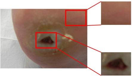
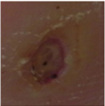
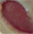
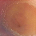
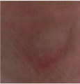
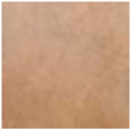
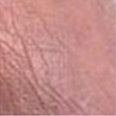
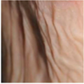
The computerized technique is used to diagnose and detect the DFU, the emerging study region with the computer vision evolution, particularly deep learning techniques. The primary research of the DFU's binary classification for regular skin is done to understand the different features of skin lesions. The new lightweight deep learning architecture is proposed in the experiment that classified the healthy skin lesions and the CNN-DFUNet with greater accuracy. In addition, the vital objective of the proposed system is to identify the skin lesion types at a higher risk of getting misclassified using algorithms. Some examples are classified correctly and incorrectly in the regular and abnormal classes using the CNN-DFUNet presented in Figure 12. The algorithms based on computer vision find it difficult to organize the subtle DFU having the same skin tone exactly. These are identified as normal, having a higher percentage than is presented in examples 1 and 2 of the cases of abnormal class misclassification. In addition, the CNN-DFUNet has a very small size, which is classified incorrectly as the normal skin lesion presented in examples 3 and 4 of the abnormal class of misclassification cases given. The patches are in the highly wrinkled skin on the toe. The very high red skin tone is misclassified and presented examples with normal classes offered (Figure 13).
Figure 12. Predicted DFU
|
Correctly classified samples as an abnormal instance |
||||||
|
Normal-68% Abnormal-99% |
Normal-0% Abnormal-100% |
|||||
|
Wrongly classified samples as an abnormal instance |
||||||
|
Normal-79% Abnormal-20% |
Normal-83% Abnormal-16% |
|||||
|
Correctly classified samples as a normal instance |
||||||
|
Normal-100% Abnormal-0% |
Normal-89% Abnormal-10% |
|||||
|
Wrongly classified samples as a normal instance |
||||||
|
Normal-15% Abnormal-84% |
Normal-26% Abnormal-73% |
|||||
Figure 13. Classified results
With the adoption of computer vision approaches, it is optimal to have different types of images to construct the dataset. Configurations with various other cameras are not allowed, and the implementations are captured with the camera. The proposed model attains superior performance with 95% sensitivity, 93% specificity, 94% precision, 95% accuracy, 95% F-measure, 97% AUC, 0.0030 SE and CI is 0.96-0.97. The proposed model works well in classifying ulcers, and its robustness is tested. The experimentation is tested for skin patches, i.e., wrinkles, spots, and normal. There is no freely accessible dataset, and with the given dataset, the skin patches are delineated with diverse patches. The best-suited CNN variants are used for comparison, and the proposed CNN-DFUNet model outperforms the existing approaches with a 5-fold CV. DL does not work effectually over the smaller dataset; however, the proposed model uses a larger filter size with parallel processing to extract huge features, making the model more efficient than others. Also, the computational complexity is considered. The algorithms for multiplying two integers with n digits have a computational complexity of $O\left(n^2\right)$, whereas the two numbers have a computational complexity of $\Theta(n)$. As a result, owing to dealing with float values with 16 decimal digits, multiplication is the most time-consuming part of the implementation procedure.
Different classifiers are trained in the proposed system depending on the conventional ML algorithms, CNN-DFUNet on the classification of DFU, the CNNs, and the suggested new architecture of CNN that differentiates the DFU skin from the normal skin. CNN-DFUNet permits the automated recognition of DFU accurately in the foot images with higher performance metrics in classification and allows it a new approach to evaluating the medical treatment and DFU. It is essential to identify the variation between healthy skin and the DFU to detect the DFU and identify the feature differences between the two classes from computer vision. The technology can transform diabetic foot ulcer detection and treatment in the proposed system, potentially turning to a paradigm shift in diabetic foot clinical care. The future goals are achieved in the proposed method based on (i) the automatic annotator is developed that is used to delineate automatically, and the foot images are classified with no need of clinicians, and (ii) the detection, recognition, and segmentation of automatic ulcer is developed using the classifiers, (iii) the method is implemented for identifying the different DFUs' pathologies like the multi-class classification is same as the classification of Texas, and few scales of grading, (iv) different user-friendly software tools are implemented that has the mobile applications to recognize the ulcer. The proposed system is used to classify skin lesions like wound classification, infections like shingles or chickenpox, and other skin lesions such as freckles, moles, pimples, and spotting marks over the normal skin, since the CNN-DFUNet performed well for the classification of DFU. CNN-DFUNet is the lightweight CNN structure utilized for the DFU dataset for classification with two classes, normal skin and ulcer. The dataset of facial skin has three classes: normal skin, spots, and wrinkles. It is further tested for including more courses in the future. Henceforth, the process of minimizing the count of neurons and the count of layers in the FC layers is demonstrated with the help of the indicated CNN-DFUNet architecture, which minimizes the processing time. On the other hand, higher specificity and higher sensitivity are obtained.
[1] Wang, L., Pedersen, P.C., Agu, E., Strong, D.M., Tulu, B. (2016). Area determination of diabetic foot ulcer images using a cascaded two-stage SVM-based classification. IEEE Transactions on Biomedical Engineering, 64(9): 2098-2109. https://doi.org/10.1109/TBME.2016.2632522
[2] Goyal, M., Reeves, N.D., Davison, A.K., Rajbhandari, S., Spragg, J., Yap, M.H. (2018). Dfunet: Convolutional neural networks for diabetic foot ulcer classification. IEEE Transactions on Emerging Topics in Computational Intelligence, 4(5): 728-739. https://doi.org/10.1109/TETCI.2018.2866254
[3] Shelhamer, E., Long, J., Darrell, T. (2017). Fully convolutional networks for semantic segmentation. IEEE Transactions on Pattern Analysis and Machine Intelligence, 39(4): 640-651. https://doi.org/10.1109/TPAMI.2016.2572683
[4] Badrinarayanan, V., Kendall, A., Cipolla, R. (2017). Segnet: A deep convolutional encoder-decoder architecture for image segmentation. IEEE Transactions on Pattern Analysis and Machine Intelligence, 39(12): 2481-2495. https://doi.org/10.1109/TPAMI.2016.2644615
[5] Perez, L., Wang, J. (2017). The effectiveness of data augmentation in image classification using deep learning. arXiv Preprint arXiv: 1712.04621. https://doi.org/10.48550/arXiv.1712.04621
[6] El-Sappagh, S., Elmogy, M., Riad, A.M. (2015). A fuzzy-ontology-oriented case-based reasoning framework for semantic diabetes diagnosis. Artificial Intelligence in Medicine, 65(3): 179-208. https://doi.org/10.1016/j.artmed.2015.08.003
[7] Fernandes, B., Vicente, H., Ribeiro, J., Analide, C., Neves, J. (2018). Evolutionary computation on road safety. In International Conference on Hybrid Artificial Intelligence Systems. Springer, Cham, pp. 647-657. https://doi.org/10.1007/978-3-319-92639-1_54
[8] Erkaymaz, O., Ozer, M., Perc, M. (2017). Performance of small-world feedforward neural networks for the diagnosis of diabetes. Applied Mathematics and Computation, 311: 22-28. https://doi.org/10.1016/j.amc.2017.05.010
[9] Hazenberg, C.E., van Netten, J.J., van Baal, S.G., Bus, S.A. (2014). Assessment of signs of foot infection in diabetes patients using photographic foot imaging and infrared thermography. Diabetes Technology & Therapeutics, 16(6): 370-377. https://doi.org/10.1089/dia.2013.0251
[10] Van Netten, J.J., Prijs, M., van Baal, J.G., Liu, C., van Der Heijden, F., Bus, S.A. (2014). Diagnostic values for skin temperature assessment to detect diabetes-related foot complications. Diabetes Technology & Therapeutics, 16(11): 714-721. https://doi.org/10.1089/dia.2014.0052
[11] Wannous, H., Lucas, Y., Treuillet, S. (2010). Enhanced assessment of the wound-healing process by accurate multiview tissue classification. IEEE Transactions on Medical Imaging, 30(2): 315-326. https://doi.org/10.1109/TMI.2010.2077739
[12] Papazoglou, E.S., Zubkov, L., Mao, X., Neidrauer, M., Rannou, N., Weingarten, M.S. (2010). Image analysis of chronic wounds for determining the surface area. Wound Repair and Regeneration, 18(4): 349-358. https://doi.org/10.1111/j.1524-475X.2010.00594.x
[13] Anthimopoulos, M., Christodoulidis, S., Ebner, L., Christe, A., Mougiakakou, S. (2016). Lung pattern classification for interstitial lung diseases using a deep convolutional neural network. IEEE Transactions on Medical Imaging, 35(5): 1207-1216. https://doi.org/10.1109/TMI.2016.2535865
[14] Yap, M.H., Pons, G., Marti, J., Ganau, S., Sentis, M., Zwiggelaar, R., Davison, A.K., Marti, R. (2017). Automated breast ultrasound lesions detection using convolutional neural networks. IEEE Journal of Biomedical and Health Informatics, 22(4): 1218-1226. https://doi.org/10.1109/JBHI.2017.2731873
[15] Tajbakhsh, N., Shin, J.Y., Gurudu, S.R., Hurst, R.T., Kendall, C.B., Gotway, M.B., Liang, J. (2016). Convolutional neural networks for medical image analysis: Full training or fine tuning? IEEE Transactions on Medical Imaging, 35(5): 1299-1312. https://doi.org/10.1109/TMI.2016.2535302
[16] Platt, J.C. (1999). Fast training of support vector machines using sequential minimal optimization. Advances in Kernel Methods, 185-208.
[17] Iandola, F., Moskewicz, M., Karayev, S., Girshick, R., Darrell, T., Keutzer, K. (2014). Densenet: Implementing efficient convnet descriptor pyramids. arXiv Preprint arXiv: 1404.1869. https://doi.org/10.48550/arXiv.1404.1869
[18] Yap, M.H., Chatwin, K.E., Ng, C.C., Abbott, C.A., Bowling, F.L., Rajbhandari, S., Boulton, A.J.M., Reeves, N.D. (2018). A new mobile application for standardizing diabetic foot images. Journal of Diabetes Science and Technology, 12(1): 169-173. https://doi.org/10.1177/1932296817713761
[19] Hermans, M.H. (2010). Wounds and ulcers: Back to the old nomenclature. Wounds, 22(11): 289-293.
[20] Foltynski, P., Wojcicki, J.M., Ladyzynski, P., Migalska-Musial, K., Rosinski, G., Krzymien, J., Karnafel, W. (2011). Monitoring of diabetic foot syndrome treatment: Some new perspectives. Artificial Organs, 35(2): 176-182. https://doi.org/10.1111/j.1525-1594.2010.01046.x
[21] Chen, X., Weng, J., Lu, W., Xu, J., Weng, J. (2017). Deep manifold learning combined with convolutional neural networks for action recognition. IEEE Transactions on Neural Networks and Learning Systems, 29(9): 3938-3952. https://doi.org/10.1109/TNNLS.2017.2740318
[22] Shi, W., Gong, Y., Tao, X., Wang, J., Zheng, N. (2017). Improving CNN performance accuracies with min-max objective. IEEE Transactions on Neural Networks and Learning Systems, 29(7): 2872-2885. https://doi.org/10.1109/TNNLS.2017.2705682
[23] Shi, W., Gong, Y., Tao, X., Zheng, N. (2017). Training DCNN by combining max-margin, max-correlation objectives, and correntropy loss for multilabel image classification. IEEE Transactions on Neural Networks and Learning Systems, 29(7): 2896-2908. https://doi.org/10.1109/TNNLS.2017.2705222
[24] He, K., Zhang, X., Ren, S., Sun, J. (2015). Spatial pyramid pooling in deep convolutional networks for visual recognition. IEEE Transactions on Pattern Analysis and Machine Intelligence, 37(9): 1904-1916. https://doi.org/10.1109/TPAMI.2015.2389824
[25] Denial, B., Shakibi, L., Dinh, M., Ranzato, de Freitas, N. (2013). Predicting parameters in deep learning. In Advances in Neural Information Processing Systems (NIPS), pp. 2148-2156. https://www.cs.ox.ac.uk/publications/publication7203-abstract.html.
[26] Greff, K., Srivastava, R.K., Koutník, J., Steunebrink, B. R., Schmidhuber, J. (2016). LSTM: A search space odyssey. IEEE Transactions on Neural Networks and Learning Systems, 28(10): 2222-2232. https://doi.org/10.1109/TNNLS.2016.2582924
[27] Cheng, J., Wu, J., Leng, C., Wang, Y., Hu, Q. (2017). Quantized CNN: A unified approach to accelerate and compress convolutional networks. IEEE Transactions on Neural Networks and Learning Systems, 29(10): 4730-4743. https://doi.org/10.1109/TNNLS.2017.2774288
[28] Li, W.J., Wang, S., Kang, W.C. (2016). Feature learning based deep supervised hashing with pairwise labels. arXiv:1511.03855. https://doi.org/10.48550/arXiv.1511.03855
[29] Huang, Z., Liu, L., van der Maaten, L., Weinberger, K.Q. (2017). Densely connected convolutional networks. arXiv:1608.06993. https://doi.org/10.48550/arXiv.1608.06993
[30] Zhou, B., Lapedriza, A., Xiao, J., Torralba, A., Oliva, A. (2014). Learning deep features for scene recognition using places database. Advances in Neural Information Processing Systems, 27. https://dspace.mit.edu/handle/1721.1/96941