Kheira Laazab*![]() | Nadjia Benblidia
| Nadjia Benblidia![]() | Ali Baaloul
| Ali Baaloul![]()
© 2025 The authors. This article is published by IIETA and is licensed under the CC BY 4.0 license (http://creativecommons.org/licenses/by/4.0/).
OPEN ACCESS
Lumbar spine disorders are prevalent conditions that can lead to chronic pain and reduced quality of life, often requiring accurate diagnosis through magnetic resonance imaging. However, manual interpretation of MRI scans is time-intensive and may lead to diagnostic errors due to the complexity of spinal anatomy and subtle differences between healthy and pathological tissues. This study aims to develop an automated method for segmenting and classifying the lumbar spine, including the assessment of lumbar lordosis, using deep learning techniques. In the first stage, spinal segmentation is performed using a combination of image thresholding and a convolutional neural network based on the U-Net architecture, with binary conversion of ground truth images and data augmentation techniques to enhance the dataset. The data is divided into training and testing sets, with 80% allocated for model training. In the second stage, classification of lumbar lordosis is achieved through a method called “Deteclordose” and transfer learning, following the automatic calculation of the Cobb angle. Images are then categorized into three classes: hyper lordosis, hypo lordosis, and normal lordosis. The method was evaluated on a dataset of MRI images obtained from Jordanian hospitals, achieving promising results, including a segmentation accuracy of 99.30%, a loss value of 0.025, a classification accuracy of 96%, a recall of 94%, and an F1 score of 93%. These outcomes demonstrate the potential of the proposed approach to improve diagnostic accuracy and reduce the burden on radiologists by providing a reliable, automated system for analyzing lumbar spine MRI images.
segment the lumbar spine, u-net, lordosis, Cobb method, classification of lumbar, lordosis, detect lordosis, transfer learning
The spine is the basic pillar of the body and consists of intervertebral and vertebral discs that intersect with the spinal cord of the central nervous system [1].
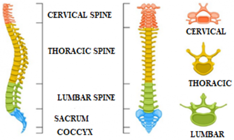
The structure of the spine can be divided into four parts. The upper part of the neck consists of 7 vertebrae called cervical, followed by 12 thoracic vertebrae, in the third part we find 5 lumbar vertebrae, and the fourth part ends at the bottom of the spine with the coccyx and sacrum [2]. as shown in Figure 1.
Figure 1. Model of a human spine [3]
Damage to its components may lead to pain or hemiplegia and may even lead to death in the case of late diagnosis. Spinal diseases are becoming more common. It is diagnosed using different techniques, and one of the most common techniques for this disease is using an MRI of the spine [1]. Magnetic resonance imaging is used to accurately diagnose pain, deformity, or curvature in the spinal canal, and it is required before surgery on the nerve axis [4]. MRI is also used to examine nerve channels [5]. Magnetic resonance imaging (MRI) has helped doctors and surgeons detect spinal diseases early and accurately. It is considered one of the most effective imaging techniques for diagnosing degenerative spinal conditions [6]. However, it requires highly qualified specialists to detect the spine, due to the similarity and closeness of the structure of the internal tissues in the magnetic resonance images. For diagnosis with a large amount of data quickly and accurately to avoid any medical error that may lead to paralysis and in some cases death, and for early treatment such as scoliosis and lumbar lordosis. Lumbar lordosis is an inward curvature of the lumbar region of the spine with curvature of the intervertebral discs and lumbar vertebrae [7]. One of the best solutions is to segment and classify the spine from MRI images using segmentation and classification techniques [8]. Segmentation of medical images is the process of separating them into several non-overlapping and homogeneous parts. Thanks to the segmentation of medical images, the diagnosis of most diseases in which magnetic resonance imaging or CT is used has become more rapid and accurate [9]. Classification of medical images is the process of diagnosing a type of disease. In recent years, artificial intelligence technologies have brought about a scientific revolution in the field of medical imaging. It helped specialists and doctors detect various diseases early and quickly. And with large amounts of data. However, it lacks accuracy and efficiency. The objective of our research is to help doctors diagnose lumbar spinal diseases accurately and quickly. This is done by developing a platform that segments the lumbar spine and classifies lumbar lordosis from MRI images using deep learning techniques.
The current work proposes to explore ways to improve deep learning techniques, specifically U-net models, to accurately and efficiently segment the lumbar spine from MRI images, and the Deteclordose model to classify lumbar lordosis from MRI images to aid in early and accurate diagnosis. For diseases of the spine. It is guided by the main research question: How can deep learning techniques improve spinal segmentation and lumbar lordosis classification from MRI images, thus helping in early and accurate diagnosis of spinal diseases?
Our contributions include:
Segmentation of the spine from MRI images
Classification of lumbar lordosis from MRI images
Our research is organized according to the following approach: Part II contains some previous works on the methods used to segment the lumbar spine and methods for classifying lumbar lordosis. The third part provides details of the different stages of the proposed model with a discussion of the data set. we find the interpretation and analysis of the results in the fourth part, and our research ends with a conclusion found in the fifth section.
Segmenting and classification of the spine from medical images is necessary for early detection and rapid diagnosis of various diseases related to it. In recent years, with the advancement of technology, various methods for segmenting and classifying the vertebrae of the spine have emerged, including semi-automatic and automated approaches based on deep learning algorithms.
2.1 Semi-automatic methods
We find in the literature that Ben Ayed et al. [11] proposed a model for dividing the vertebrae of the spine, based on the graph cut method, through two stages. first, placing three points on each vertebra, then calculating the model distribution to separate the boundaries of each vertebra from its adjacent structures. Zukic et al. [12]. developed from the approach of Viola and Jones (2001), which relies on identifying the vertebrae of the spine and determining the center of the vertebrae. from there, the spinal vertebrae were segmented frequent inflation method. the results of the division also led to the classification of spinal diseases into three diseases. Hille et al. [13] developed a hybrid-level method to segment the vertebral body. this was done in stages. first, the center and size of the vertebrae were determined by placing three marks on each vertebra and then defining a vertebra using a cylinder. based on filtering by morphological methods and density information, the vertebral body was segmented. Altini et al. [14] segmentation combined with machine learning algorithms k-NN, k-means, and deep learning CNN to identify and segment spinal vertebrae. first, v-net [15]. Semantic segmentation is used to identify the backbone. then, determine the number and type of paragraphs to be divided by placing dots in the center of each paragraph. finally, using k-NN, the paragraphs are segmented. This approach was applied to the verse 2020 dataset and achieved a DSC of 0.90. However, this model requires greater precision.
2.2 Automatic methods
We also find some litterateurs rely on automated methods using artificial intelligence algorithms.
Janssens et al. [16] proposed an approach to segmenting the lumbar spine, which goes through two stages: first, localizing the lumbar spine using a three-dimensional FCN, then cutting the lumbar region from an image and training it on a second FCN network to segment the lumbar spine accurately. Their model achieved excellent results of 95%. The FCN method was used to tag and segment vertebrae [17]. This combines the memory component of the vertebral information with the network, and after segmentation, it searches for a neighboring vertebra to process it. FCN results were good, with one vertebra with a Dice Similarity Coefficient of 93%. Klein et al. [18], A method to identify and segment vertebrae from computed tomography images using a convolutional neural network (CNN) method, based on the graph convolutional network (GCN), which identified the vertebrae by marking the structure. Möller et al. [19] Their approach is organized into two distinct phases. First, the semantic model uses the nnUNet architecture to divide the scan into 14 semantic labels. Then, using a sliding window technique, a secondary model distinguishes semantic labels in vertebrate instances, taking advantage of the center of mass placements. The predictions are then unified through dice score calculations and organized into triplets to mitigate discrepancies. Kawathekar and Aparna [20], propose a method for segmenting the spine based on three stages: first to determine the center of the spine, then develop the Unbalanced-UNet deep learning algorithm, then mark the vertebrae using the Spatial Configuration Network (SCN), and finally the U-Net network for segmenting the vertebrae. Their approach was applied to the VERSE'19 database, achieving an accuracy rate of 93.07%.
As for cases of hyper lordosis / straight back / flat back, both were shown by Masood et al. [21] in a smaller area (Ar) compared to normal lordosis, while cases of excessive lordosis/backswing showed a larger area, consistent with previous results. The automated classification system for spinal disorders achieved an accuracy rate of 93\% in distinguishing these conditions from normal lordosis. Furthermore, the study provides an enhanced measure of angular deviation for classifying spondylolisthesis and suggests the use of centroid-based area calculations instead of traditional angular points for spine assessment.
Maraş et al. [22] used pre-trained deep learning techniques, such as DenseNet-201, Resnet-101, VGG-19, and VGG-16, to classify cervical normality, mechanical neck diseases, cervical degenerative disc disease, and osteoporosis, after performing a series of operations on a group of Data from increasing the number of data, adjusting the dimensions, and dividing the data set into training, validation, and testing. Their study was applied to 170 lateral radiographs of osteoporosis with cervical osteoporosis and cervical degenerative disc disease. And 161 lateral radiographs of the normal cervix, and achieved the accuracy rate of VGG-16 and VGG-19, Resnet-101, and DenseNet-201 are 93.9%, 91.8%, 89.8%, and 85.7%, respectively. These are acceptable percentages but need more scrutiny. Johnson et al. [5] developed a method that helps in diagnosing lordosis by calculating the area of a closed region located between S and L1, and the line that connects L1 to L2, L2 to L3, L3 to L4, L4 to L5, and L5 to S. He placed an obstacle between an angle Lordosis and the area of the closed part, to classify lordosis diseases.
2.3 Our position
Based on the above review, further research must address the need for more efficient and accurate spine segmentation and classification techniques, which play a vital role in enhancing early disease detection and diagnosis. Despite the progress in AI-driven approaches, there remains a need to streamline localization processes and improve segmentation accuracy to facilitate better clinical outcomes.
Segmenting the lumbar spine from MRI images is an important step in classifying lumbar lordosis in medical images. To achieve this, it is necessary to rely on a methodology that uses specific methods in a special applied environment, which work to segment the lumbar spine and classify the type of lumbar lordosis, as shown below:
3.1 Material
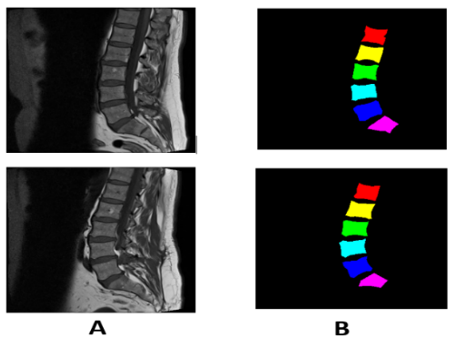
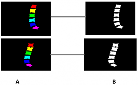
The data sets are a set of MRI images collected at Irbid Specialist Hospital in Jordan between September 2015 and July 2016 [14]. For people suffering from spinal diseases, it consists of 514 image sections of the lumbar spine, and this is after ignoring some images that were not clear due to noise [23]. Published on Mendeley Data [21]. The datasets contain 514 topics with ground truth labels, containing false color segmentation and pixel labels [1]. Ground truth labels are denoted by L1, L2, L3, L4, L5, and S [16]. All images have dimensions of 320*320. Some images of the data set are shown in Figure 2.
Figure 2. (A) Sagittal images of the spine (B) It represents ground truth images with colors
3.2 Methods
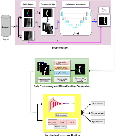
To segment and classify lumbar spine lordosis in an accurate, fast, and simple way. We propose our approach. It first relies on segmenting the lumbar spine from MRI images based on a deep learning algorithm and thresholding method. This is done in two basic steps. First, we prepared the dataset by converting ground truth color images into binary images using a thresholding method. We applied a set of geometric operations to augment the dataset and partition the medical MRI dataset to train and test the model. Then, we modified the U-Net model by changing the size of the filters and increasing the number of layers and obtained the backbone segmentation. Second, classify lumbar lordosis using a deep learning model. It was built based on CNN and some trained models after preparing the dataset through and lumbar lordosis angle (LLA) calculation using the Cobb method. Then classify they were classified into three categories: hyper lordosis, normal, and hypo lordosis. Figure 3 shows a schematic diagram of the proposed model. The proposed method for segmenting the lumbar spine and classifying the curvature can be summarized in Figure 4.
Figure 3. Techniques used for lumbar spine segmentation and lordosis classification
Figure 4. Overview of the approaches proposed for lumbar lumber spine segmentation and classification of lordosis
3.3 Segmentation of lumbar spine data
The stage of segmenting the lumbar spine from MRI images is an important step in diagnosing diseases such as lumbar lordosis. It is a difficult task due to the similarity of the internal structure of the tissues. Therefore, we proposed an approach that focuses on the following stages:
3.3.1 Prepare spinal data
This stage is considered a basic stage in our model. It aims to convert ground truth color images into binary. Thresholding is the simplest method. The calculation time can be minimized a more evaluation of the lumbar spine. This work utilizes a threshold for segmenting images [24]. This is done by testing each pixel of the image to see if its value is above or below a certain threshold and producing a binary image that combines the results. There are several ways to automatically detect the threshold value to apply. One of the most widely used methods is the Otsu method [25]. The automatic threshold value is determined using the OTSU method based on the shape of the image histogram. This method requires pre-calculation of the image histogram to obtain a binary image containing only two categories (lumber, spinal and background) [26]. We determine the ideal threshold T that separates these two classes through an iterative algorithm such that the maximum is the variance between the classes, and the minimum is the variance within the class [27].
This stage can be summarized in Algorithm 1.
|
Algorithm 1: Segmentation Using Global Thresholding |
This value distinguishes the foreground from the background in a grayscale image. It can be determined either manually or through automated methods such as Otsu's algorithm.
The selected threshold is applied to the grayscale image. The outcome is a binary mask M(x,y). defined in Eq. (1), which identifies the segmented areas. $M(x, y)=f(x)=\left\{\begin{array}{l}1 \,\, { if }\,\, I(x, y)>T h \\ 0 \quad { othewise }\end{array}\right.$ (1) I (x,y) is the grayscale intensity at pixel (x,y), This is the chosen threshold. The binary mask M(x,y) highlights the foreground with pixel values of 1, while background areas are assigned a value of 0. |
3.3.2 Data augmentation
Deep learning models perform better when trained on large datasets. However, when only a small amount of data is available, data augmentation can help improve performance by increasing the variety of training examples [28].
In this work, we applied several geometric transformations to expand both the training and testing datasets. These transformations, shown in Table 1, include image rotation, vertical flipping, and horizontal flipping. This approach helps reduce overfitting and improves the model’s ability to generalize.
Table 1. Geometric operations applied to increase the number of data, mentioning the field and unit of measurement
|
Operation |
Interval/Valeur |
Unite |
|
Rotate |
$\left[-45^0,+45^0\right]$ |
Degré |
|
Horizontal |
$[-\pi,+\pi]$ |
Radian |
|
Vertical |
$[-\pi,+\pi]$ |
Radian |
3.3.3 Lumbar spine segmentation
The method adopted for segmenting the lumbar spine from MRI images is based on a Fully Convolutional Network (FCN) of the encoder–decoder type, using the U-Net architecture [29]. We introduced a set of architectural modifications to the original U-Net model by employing an encoder–decoder structure composed of 23 layers: 10 in the encoder and 13 in the decoder. The network consists of 18 convolutional layers and 4 deconvolutional layers. The increase in the number of layers was aimed at enabling the network to learn more complex and fine-grained features, which is crucial given the anatomical intricacies present in MRI images. All convolutional and deconvolutional layers used filters of size (3×3), a standard choice that offers an optimal balance between computational efficiency and the ability to capture local spatial patterns in medical images. In the encoder, the number of filters was gradually increased: 16 filters in the first two layers, followed by 32, then 64, 128, and finally 256 filters in the last two layers. This design enables multi-level feature abstraction, from low-level details to higher-level semantic representations. The decoder mirrored this progression in reverse, using blocks that combine convolutional and deconvolutional layers: starting with 128 filters, then 64, and finally 32 filters in the last block. Deconvolutional layers were employed to enhance the spatial resolution of the segmented output and better preserve boundary details compared to standard upsampling techniques. The ReLU activation function was applied throughout to accelerate training, prevent the vanishing gradient problem, and promote efficient nonlinear learning. The Adam optimizer was chosen for its stability and adaptive learning capabilities, with a learning rate set to 0.001 and a batch size of 16. These hyperparameters were selected after extensive experimentation with different data split ratios, epoch counts, and optimizer configurations. Overall, the proposed architectural enhancements, including the systematic use of 3×3 filters, have proven effective in improving segmentation performance for the targeted anatomical regions. The various stages of the U-Net architecture of our model are represented in Figure 5.
3.4 Prepare spinal data for classification
This stage is considered important before the classification of lumbar lordosis from MRI images, is focuses on the following stages:
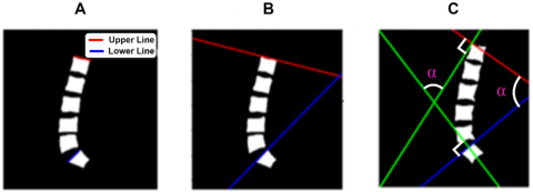
3.4.1 Measurement of lumbar lordosis angle
After segmenting the lumbar spine from the MRI images, we determined the angle LLA between the superior endplate S and the superior endplate L1. Using the Cobb method, the angle LLA was calculated to calculate the Cobb angle between the upper limb S and the upper limb L1, i.e., calculate the LLA. We must follow the following steps [29].
$M_{(L 1, s)}=\frac{Y_{2 y}-Y_{1 y}}{X_{2 y}-X_{1 y}}$ (2)
M represents the slope of the lines,
Y1y and Y2y: represent the rank on the y-axis
X1x and X2x: represent a comma on the x-axis.
$angle =tan ^{-1}\left|\frac{M_{L 1}-M_S}{1+M_{L 1} M_S}\right|$ (3)
$M_{L 1}$: is the slope of the L1 line,
$M_S$: is the slope of the line S.
Figure 5. Model architecture for U-net the lumbar spine segmentation
Figure 6. Spinal angular cobb measurements
3.4.2 Automated lumbar lordosis classification
After calculating the LLA angle using the Cobb method, we classified the data set into three categories based on the angle measurement, where the typical range of normal lumbar lordosis (LLA) angle extends from 39° to 53° [30]. It falls within Category 1, while angles greater than 53 degrees fall into the category of hyperhidrosis, which is classified as Category 2. In contrast, hypohidrosis, for angles less than 39 degrees, is classified as Category 1. As shown in Algorithm 2.
|
Algorithm 2: Pseudocode for LLA Classification |
|
Begin Set LLA If α < 390 then Assign Low_Angles, Cl0, Hypolordosis Else If α < 530 Assign Medium_Angles, Cl1, Normal lordosis Else Assign High_Angles, Cl2, Hyperlordosis End If End If end |
3.4.3 Augmentation and resizing the dataset
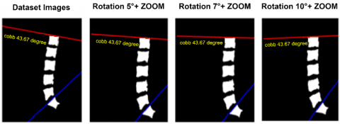
Given the limited size of our dataset (514 images), we applied geometric data augmentation techniques, including small-angle rotations (+5°, +7°, +10°) and zooming, to expand the dataset to 2056 images, as detailed in Table 2 and Figure 7. These small rotation angles were not chosen arbitrarily. In medical imaging, especially of the lumbar spine, large angles (e.g., ±90°, ±180°) often produce anatomically implausible images and can confuse the model. Conversely, small-angle rotations preserve anatomical consistency while introducing beneficial variability for training. Our choice is supported by the study by Qin et al. [31], which found the best segmentation performance at 10°, with smaller angles (5°, 10°) yielding clinically realistic results. Larger rotations (20°–30°) led to distortions that reduced model accuracy. Therefore, the use of +5°, +7°, and +10° angles in our work is both clinically relevant and empirically optimal.
Table 2. Augmentation dataset methods
|
Operation |
Itervale/Valeur |
Unite |
|
Rotation |
10 |
Degré |
|
Rotation |
5 |
Degré |
|
Rotation |
7 |
Degré |
|
Zoom |
10% |
Pixel |
Figure 7. Results of data augmentation techniques applied to images
Figure 8. Normalize and resize images
Figure 9. Architecture of the model ‘Deteclordose’
The second part at this stage is normalizing [32] and adjusting the size of the data, as the CNN model works on grayscale images, meaning that the value of each pixel is from 0 to 1. That is, the density of the images is limited to between 0 and 255, so we multiplied each image by 1/255 of the pixel value. We also adjusted the data size from 320×320 to 224×224 in the Figure 8 shows this.
3.5 Lumbar lordosis classification
The stage of classifying lumbar lordosis from MRI images after initializing a data set. It is a necessary and basic stage in our research. To establish an accurate, excellent, and fast method, we experimented with some trained deep-learning models. We also built our model based on CNN, which gave excellent efficiency and accuracy.
3.5.1 Classification of the spinal lumbar with “Deteclordose”
The proposed model is based on a convolutional neural network (CNN) architecture specifically designed for classifying images into three categories of lumbar lordosis from MRI images. This architecture is optimized to handle classification tasks with high precision while maintaining computational efficiency. The proposed model consists of six convolutional layers with 3×3 filters and ReLU activation, increasing the filters from 32 to 512 and 2×2 pooling layers to reduce complexity. The fully connected layer uses a dense layer with 128 neurons and Dropout at 50% to prevent overfitting. The output layer, with Softmax activation, classifies the images into three classes, ensuring high precision and computational efficiency. The optimal results were achieved after conducting multiple tests that involved adjusting the dataset split ratio, epoch size, batch size, learning rate, and optimizer. The best configuration included a dataset split of 80% training and 20% testing, a batch size of 32, an epoch size of 200, a learning rate of 0.001, and using the Adam optimizer [33]. The architecture of the proposed ‘Deteclordose’ model is illustrated in Figure 9.
3.5.2 Classification of the spinal lumbar with transfer learning
To know the efficiency and accuracy of the proposed model for classifying lumbar lordosis in magnetic imaging images, we exploited some pre-trained deep learning models for image classification to solve the problem of relatively small data and long training time [34], DenseNet121 [35], VGG16 [36], and VGG19 [37], were used. Table 3 shows the architectural explanation of the different models used.
Table 3. Architecture of some pre-trained models
|
Models |
Input Size |
Output Size |
No. of Layers |
|
DenseNe121 |
[224,224 ,3] |
[3, 1] |
121 |
|
VGG19 |
[224,224,3] |
[3, 1] |
19 |
|
VGG16 |
[224,224,3] |
[3, 1] |
16 |
3.6 Evaluation criteria
Our model is evaluated by calculating the precision (p) and loss error (ME), where p is the matching ratio between the segmentation regions and the ground truth images used as reference. The accuracy (precision) is calculated according to the following Eq. (4):
$P=\frac{ { real \,\,positive }}{ { total \,\,expected \,\,positive }}$ (4)
The accuracy value is limited to [0,1]. The better the segmentation and classification, the greater the accuracy.
ME represents the loss error between the expected ground and truth values. The lower the ME percentage, the more accurate the result will be.
ME is calculated by Eq. (5):
$M E=\frac{1}{L} \sum_{i=0}^{L-1}\left|\left(\widehat{Y_l}\right)-Y_I\right|$ (5)
L = total number of images
i: the expected lumbar spine segment
Y: the ground truth of the lumbar spine
Precision (p) is the ratio of true positives to the total number of positive predictions. It is calculated using the formula Eq. (6):
$p=\frac{\text { True Positives }}{\text { Total Positive Predictions }}$ (6)
Recall (R), also known as the true positive rate or sensitivity, is the quotient of the true positives by the sum of the true positive and false negatives. It is calculated using the relation Eq. (7):
$R=\frac{\text { True Positives }}{\text { True Positives }+ \text { False Negatives }}$ (7)
F1score is the harmonic average of recall and precision. Thanks to it a scale is provided that weighs between both scales. It is calculated by the relation Eq. (8):
$F1score=\frac{2 \times(\mathrm{P} \times \mathrm{R})}{\mathrm{P}+\mathrm{R}}$ (8)
3.7 Overfitting mitigation strategies
Given the relatively small size of the dataset (514 images), several strategies were employed to reduce the risk of overfitting and ensure the model’s generalization capability. Thèse include:
While these measures help mitigate overfitting.
3.8 Environment experimental
Our model was implemented in Python, using TensorFlow, which is an image-processing library. First, in the stage of preparing the spinal data, we used Jupyter, and to divide the database, we used Spyder in Anaconda, and this was on a laptop equipped with a fast Intel(R) Core (TM) i7-6500U processor. 2.50 GHz, 2601 MHz core, 4 logical processors, and RAM. 8.00 GB installed. Train U-Net was done on a colab platform with a type of processor GPU.
Different deep-learning methods were used to segment and classify the lumbar spine in a dataset to improve and increase the accuracy of diagnosis.
4.1 Segmentation spine lumbar
Deep learning technology was applied to the dataset. This is after converting the color ground images into binary images using the thresholding method, where the threshold value was set to 82.08, which was determined by Otsu, which is the dividing value between the two categories: the lumbar spine and the background of the image. We then applied geometric techniques to increase the Amount of data. Finally, we trained the model to segment the lumbar spine.
Figure 10 represents some of the colored ground truth images and their conversion into binary images. This is after setting the threshold value of 82.08 so that we obtain an image with two categories; the value greater than the threshold value represents the lumbar spine, and the value less than the threshold value represents the background of the image.
Figure 10. Normalize the images
After applying operations to the augmentation dataset, 2036 images were obtained out of 509 images. Figure 11 shows some of the images to which geometric operations to augmentation.
Figure 11. Normalize and resize images
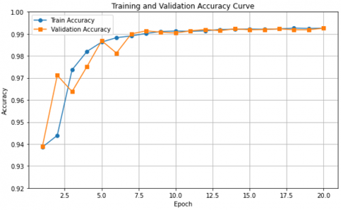
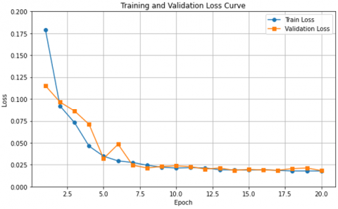
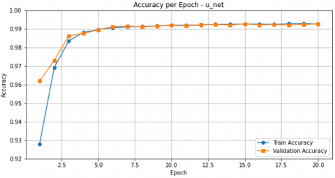
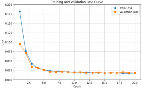
The curves of Figure 12 and Figure 13 show a graphical representation of the change in the training accuracy result and the validation training loss result, respectively, as a function of 20 epochs divided into 30% testing and 70% training.
We notice that the accuracy percentage increases to 99.20%, and starting from the eighth epoch, the two curves begin to match, as shown in Figure 12. We notice that the loss rate decreases to 0.02% in Figure 13, and the two curves match starting from the eighth epoch.
Figure 12. Training and validation accuracy result (30% testing and 70% training)
The curves of Figure 14 and Figure 15 show a graphical representation of the change in the training accuracy result and the validation training loss result, respectively, as a function of 20 epochs divided into 20% testing and 80% training. We notice that the accuracy percentage increases to 99.30% accuracy, and starting from the Third epoch, the two curves begin to match, as shown in Figure 14. We notice that the loss rate decreases to 0.025% in Figure 15, and the two curves match starting from the third epoch. These are good results compared to the results of the division (30% testing and 70% training), which showed an overfit in the results, which led to the loss of some information about the shape of the spinal vertebrae, in contrast to the results of the division (20% testing and 80% training).
Figure 13. Training and validation loss result (30% testing and 70% training)
Figure 14. Training and validation accuracy result (20% testing and 80% training)
Figure 15. Training and validation loss result (20% testing and 80% training)
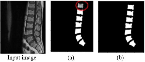
We noticed in Figure 16 that there was overfitting in the results, which led to the loss of some information, which appeared in the form of a missing part in the spine segmentation image, as shown by the circle in Figure 16(a), in contrast to the results of u_net, where the results were good and appear This is due to the accuracy of the segmentation of the spinal vertebrae, which appeared clearly as shown in Figure 16(b).
Figure 16. (a) prediction with 30% test and 70% training, (b) prediction resulting with 20% test and 80% training
4.2 Comparison of the model’s segmentation
The comparison between our proposed methodology and previous approaches demonstrates its superior effectiveness. Our method relies on converting color ground truth images into binary masks using thresholding and the Otsu method, followed by accurate segmentation of the lumbar spine region from MRI images. In contrast, Sudirman et al. [1] employed a hybrid model combining YOLOv5, HED, and U-Net for vertebrae detection and segmentation. Meanwhile, Wang et al. [38] introduced an enhanced strategy based on U-Net++ to improve U-Net performance in spinal segmentation from MRI scans, with their results detailed in Table 4, and U-Net [39] stands out as one of the most effective architectures for biomedical image segmentation, due to its encoder–decoder structure and skip connections that preserve spatial information.
To assess the impact of our structural modifications, we restructured the baseline U-Net model to include 24 layers, among which 18 are convolutional, while keeping other parameters, such as kernel size, unchanged, and using the ReLU activation function in all convolutional layers. After retraining the modified model on the same dataset with a learning rate of 0.001 and a batch size of 16, it achieved an accuracy of 94.29%, which is significantly lower than that of our proposed model.
This considerable performance gap highlights the effectiveness of the architectural improvements we introduced and confirms their essential contribution to enhancing segmentation quality. Based on these results, our proposed method offers practical and valuable benefits to physicians and medical specialists by supporting diagnostic processes and facilitating the early detection of spinal disorders.
Table 4. Comparison of the results of different segmentation methods
|
Year |
Authors |
Category |
Approach |
Accuracy |
|
2022 |
Sudirman et al. [1] |
MRI |
YOLOv5-HED-UNet |
74.5% |
|
2023 |
Wang et al. [38] |
MRI |
U-Net |
86.2% |
|
2023 |
Wang et al. [38] |
MRI |
U-Net++ |
88% |
|
2025 |
This work |
MRI |
Modified U-Net |
94.29% |
|
2025 |
This work (Proposed) |
MRI |
Threshold + U-Net |
99.3% |
4.3 Classification of lordosis lumbar
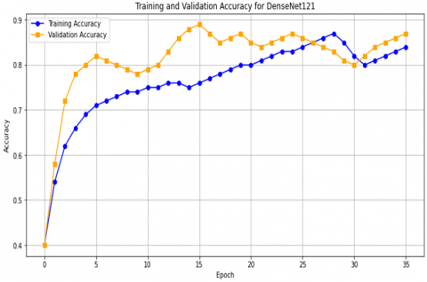
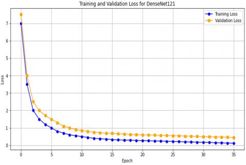
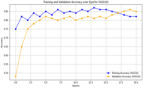
Figure 17 shows the results obtained for DenseNet121, VGG19, and VGG16 in terms of accuracy and loss as a function of the number of epochs. In Figure 17(a), we see the results for DenseNet121, where training stopped after 34 epochs due to early stopping and the accuracy reached 87%. In Figure 17(c), for VGG19, training stopped after 40 epochs out of 200, with an accuracy rate of 83%. For the VGG16 model, as shown in Figure 17(e), the accuracy reached 90% after 50 epochs.
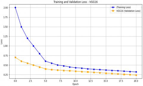
Figure 17(b) shows the loss results as a function of the number of epochs for DenseNet121, which reached 0.5%. For VGG19, as shown in Figure 17(d), the loss was 0.45%. For the VGG16 model, as shown in Figure 17(f), the loss percentage was 0.25%.
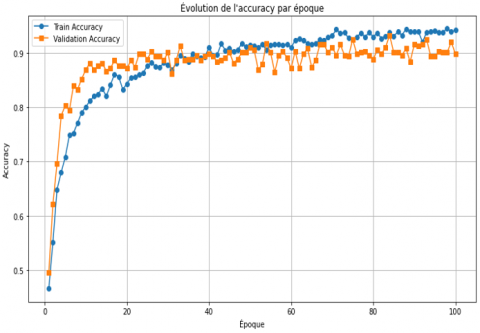
After training the Deteclordose model, the accuracy and loss results were obtained, as shown in Figure 18. In Figure 18(a), the accuracy results are shown, where the accuracy rate reached 96% after 100 epochs, which is a significant improvement compared to the previous models. In Figure 18(b), the loss rate was 0.25%, while in the Deteclordose model, the loss rate was 0.1%, which is the best result compared to the previous models.
(a) Training and validation accuracy DenseNet121 result
(b) Curve histogram of training and validation loss for DenseNet121 result
(c) Training and validation accuracy VGG19 result
(d) Curve histogram of training and validation loss for VGG19 result
(e) Training and validation accuracy VGG16 result
(f) Curve histogram of training and validation loss for VGG16 result
Figure 17. The accuracy and loss results obtained for: DenseNet121, VGG19, and VGG16
(a) Training and validation accuracy Deteclordose result
(b) Training and validation Deteclordose loss result
Figure 18. Results accuracy and loss from Deteclordose
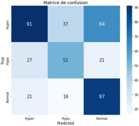
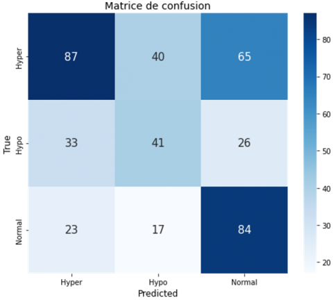
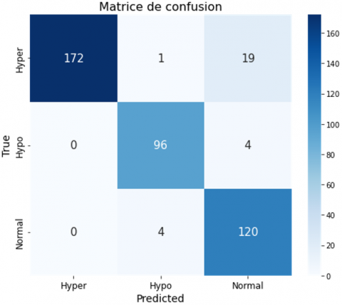
The confusion matrix evaluates the performance of the classification models “DenseNet121,” “VGG16,” “VGG19,” and “Detect LORDOSE” for three classes: “Hyper,” “Hypo,” and “Normal.” In Figure 19(a), DenseNet121 has difficulty with accuracy, especially in distinguishing between classes. In Figure 19(b), the VGG16 confusion matrix shows significant misclassifications, especially in distinguishing between the “Hyper” and “Hypo” classes. VGG19 has notable difficulties with the “Hypo” class, as shown in Figure 19(c). The Detect LORDOSE model works better overall, but still has some issues, especially in the “Normal” category. In general, as shown in Figure 19(d), it achieved the best performance compared to its predecessors.
(a) Confusion matrix DenseNet121
(b) Confusion matrix VGG16
(c) Confusion matrix VGG19
(d) Confusion matrix Deteclordose
4.4 Comparison of the model’s classification
Model Performance Comparison shows the performance of four different models for a classification task, evaluated on several metrics: accuracy, loss, precision, recall, and F1 score (Table 5). Here is a brief commentary on the results:
Table 5. Model performance comparison
|
Model |
Accuracy |
Loss |
Precision |
Recall |
F1 Score |
|
DenseNet121 |
87% |
50% |
56% |
56% |
55% |
|
VGG19 |
83% |
45% |
51% |
52% |
50% |
|
VGG16 |
90% |
25% |
52% |
53% |
53% |
|
DetecLordose |
96% |
10% |
92% |
94% |
93% |
DenseNet121: Shows a good accuracy of 87%, but its other performance metrics (precision, recall, and F1 score) are quite low (around 55-56%), indicating poor overall performance despite good accuracy. VGG19: Shows overall lower performance with an accuracy of 83% and precision, recall, and F1 score scores around 50-52%. The loss is 45%, suggesting moderate effectiveness. VGG16: Obtains a better accuracy of 90% with precision, recall, and F1 score scores slightly higher than those of VGG19 but still low (around 52-53%). The loss is relatively low at 25%.
DetecLordose: Stands out significantly from other models with an accuracy of 96%, very high precision, recall, and F1 scores (92-94%, 93% respectively), and a very low loss of 10%, indicating superior performance in all aspects assessed.
Here we analyze and compare the results of the confusion matrix for the classification model, where:
The confusion matrices for the DenseNet121, VGG16, VGG19, and Deteclordose models are shown in Figure 19.
After analyzing the confusion matrix results presented in Table 6, it is evident that the proposed model, DetectLordose, significantly outperforms the baseline models (DenseNet121, VGG19, and VGG16) in classifying the three categories: Hyperlordosis, Normal lordosis, and Hypolordosis. The model demonstrated very high accuracy, achieving high true positive (TP) rates and notably low false positive (FP) and false negative (FN) rates, particularly for the Hyperlordosis class, where no FP cases were recorded. In contrast, the DenseNet121 model struggled to distinguish between classes, with high FP and FN values, especially in the Hyper and Hypo categories. VGG19 performed slightly worse, exhibiting higher misclassification rates, likely due to overlapping visual features across classes. VGG16 showed a relative improvement over VGG19 and DenseNet121, but still suffered from notable classification errors.
These classification errors are primarily due to class imbalance in the dataset, visual and anatomical similarity between the different lordosis categories, and structural limitations of conventional models in extracting discriminative features. The error rate can be reduced through several possible solutions, such as data augmentation, class rebalancing, and improving the model architecture, to enhance classification accuracy and minimize misclassification rates. The outstanding performance of the proposed DetectLordose model is mainly attributed to its specialized design, enhanced architecture, advanced training configuration, and optimal tuning of training parameters, all of which contributed to achieving strong results.
Table 6. Detailed model performance
|
|
Hyperlordosis |
Normal-lordosis |
Hypolordosis |
|
Model |
TP FP FN TN |
TP FP FN TN |
TP FP FN TN |
|
Densenet121 |
91 48 101 176 |
87 85 37 207 |
52 53 48 263 |
|
VGG19 |
87 56 105 168 |
84 91 40 201 |
41 57 59 259 |
|
VGG16 |
109 62 83 162 |
63 65 61 227 |
52 65 48 251 |
|
Detectlordose |
172 0 20 224 |
120 23 4 269 |
96 5 4 311 |
Although model accuracy is a key performance indicator, the comparison also considered computational and practical aspects relevant to clinical deployment. Table 7 summarizes the performance and efficiency metrics of the proposed Deteclordose model compared to widely used pre-trained models (VGG16, VGG19, and DenseNet121).
The results demonstrate that Deteclordose outperforms the other models in terms of accuracy, achieving 96%, compared to 90% for VGG16 and 87% for DenseNet121. While the number of parameters in Deteclordose (23.91 million) is not the lowest, it remains within an acceptable range and is significantly lower than that of DenseNet121 (32.79 million). Furthermore, the model size (91.14 MB) is moderate—larger than VGG16 but smaller than DenseNet121—making it suitable for integration into clinical systems without requiring substantial computational resources.
In light of these findings, Deteclordose can be considered the most balanced solution, combining high accuracy with computational efficiency. This balance makes it a strong candidate for clinical applications that require reliable precision, quick response times, and deployment in environments with limited hardware capacity.
Table 7. Comparison of deep learning models based on accuracy, parameters, and model size
|
Model |
Accuracy |
Paramètres (Millions) |
Model Size (MB) |
|
VGG16 |
90% |
17.93 |
68.38 |
|
VGG19 |
83% |
23,23 |
88.58 |
|
DenseNet121 |
87% |
32,79 |
125.10 |
|
Deteclordose |
96% |
23.91 |
91.14 |
4.5 Discuss the classification results
The results indicate that the Detect model, especially with a dropout of 0.5, outperforms the other models in terms of all performance metrics. This superiority is visible in the higher values of precision, recall, and F1 score, as well as in the confusion tables, which show minimal errors. The DenseNet121, VGG19, and VGG16 models, while performing well in some metrics like accuracy, exhibit significant weaknesses in precision, recall, and F1 score, as well as higher rates of FP and FN.
4.6 Limitations and future work
Despite the promising outcomes achieved in this study, several limitations must be acknowledged. A major limitation is that the dataset was collected from a single medical institution—namely, Irbid Specialist Hospital in Jordan. This raises concerns about potential demographic bias and limits the generalizability of the findings to broader and more diverse populations. Moreover, the study did not account for variations in MRI scanner types, imaging protocols, or clinical and demographic characteristics of patients that may differ across healthcare institutions.
In addition, the proposed method has not yet been evaluated within real-world clinical workflows, such as integration with Picture Archiving and Communication Systems (PACS) or assessment by practicing radiologists. Practical implementation barriers, such as processing time and hardware requirements, were also not addressed, yet they are essential for the deployment of AI-based systems in clinical environments.
Future work should aim to incorporate multi-center datasets from diverse geographical and institutional contexts, validate the model in actual clinical settings, and optimize computational performance to ensure efficiency and real-time applicability. Furthermore, collaboration with healthcare professionals will be critical to assess the system’s clinical utility and to guide its integration into existing radiological workflows.
In our research, we proposed a model that segments the lumbar spine and classifies lumbar lordosis from MRI images. This is to help doctors and specialists in the early and rapid detection of lumbar spine diseases using deep learning algorithms. First, in order to segment the lumbar spine, we relied on the deep learning architecture of the programmer and decoder, which we designed by increasing the depth of the layer. Additionally, leveraging the Threshed and Otsu methods, we carefully prepared the dataset, converting color ground truth images into binary representations to serve as segmentation masks during model training. To enhance the accuracy, we expanded the dataset using geometric techniques applied to the images. It is worth noting that our model underwent rigorous testing on the dataset of a patient with spinal diseases, resulting in commendable effectiveness in terms of accuracy and loss, achieving an impressive result of 99.3%. To classify lumbar lordosis, we calculated the lumbar angle using the Cobb method, and then we classified the data set into three groups: hyperhidrosis/hyperhidrosis / normal lordosis, according to the angle measurement. Then we trained our proposed model called Deteclordose to classify lumbar lordosis from MRI images. Achieved an impressive score of 96%. Moving forward, our research methods extend to the segmentation and classification of pelvic, thoracic, and cervical spine pathology from MRI images, providing potential applications in the early identification of spinal deformities to alleviate the necessity of invasive surgical interventions. However, future endeavors should address limitations such as scalability and generalizability to diverse patient populations while exploring ways to improve computational efficiency and robustness in real-world clinical settings.
The MRI dataset used in this study was obtained from an open-access source and contains no personally identifiable patient information. Therefore, by the data provider’s terms of use, ethical approval and prior patient consent were not required.
The dataset [21] is freely available at the following link: https://data.mendeley.com/datasets/k3b363f3vz/2.
We reaffirm our full commitment to scientific ethics and internationally recognized standards in the use of medical imaging data.
|
MRI |
Magnetic Resonance Imaging |
|
CT |
Computed Tomography |
|
LLA |
Lumbar Lordosis Angle |
|
FCN |
Fully Convolutional Network |
|
CNN |
Convolutional Neural Network |
|
ReLU |
Rectified Linear Unit (activation function) |
|
Th |
Threshold |
|
VGG19 |
Visual Geometry Group 19-layer network |
|
VGG16 |
Visual Geometry Group 16-layer network |
|
DenseNet121 |
Densely Connected Convolutional Network with 121 layers |
|
YOLOv5 |
You Only Look Once, version 5 – a real-time object detection model known for speed and accuracy |
|
HED |
Holistically-Nested Edge Detection – a deep network for detecting semantic edges in images |
|
U-Net |
Convolutional network architecture for biomedical image segmentation with encoder-decoder structure and skip connections |
|
U-Net++ |
Enhanced version of U-Net with nested and dense skip connections for better feature fusion |
[1] Sudirman, S., Kafri, A.A., Natalia, F., Meidia, H., Afriliana, N., Al-Rashdan, W. (2019). MATLAB source code for developing ground truth dataset, semantic segmentation, and evaluation for the lumbar spine MRI dataset. Mendeley Data.
[2] Bolton, R., Hulshof, H., Daanen, H.A., van Dieën, J.H. (2022). Effects of mattress support on sleeping position and low-back pain. Sleep Science and Practice, 6(1): 3. https://doi.org/10.1186/s41606-022-00073-x
[3] Freepik. https://www.freepik.com/free-vector/spine-structure-anatomy-composition-with-colored-view-spine-divisions-with-editable-text-captions-vertebrae-vector-illustration_64993434.htm.
[4] Ng, S.Y., Bettany-Saltikov, J. (2017). Imaging in the diagnosis and monitoring of children with idiopathic scoliosis. The Open Orthopaedics Journal, 11: 1500. https://doi.org/10.2174/1874325001711011500
[5] Johnson, M.A., Gohel, S., Mitchell, S.L., Flynn, J.J.M., Baldwin, K.D. (2021). Entire-spine magnetic resonance imaging findings and costs in children with presumed adolescent idiopathic scoliosis. Journal of Pediatric Orthopaedics, 41(10): 585-590. https://doi.org/10.1097/BPO.0000000000001943
[6] Modic, M.T., Ross, J.S. (2007). Lumbar degenerative disk disease. Radiology, 245(1): 43-61. https://doi.org/10.1148/radiol.2451051706
[7] Been, E., Kalichman, L. (2014). Lumbar lordosis. The Spine Journal, 14(1): 87-97. https://doi.org/10.1016/j.spinee.2013.07.464
[8] Tang, X. (2019). The role of artificial intelligence in medical imaging research. BJR| Open, 2(1): 20190031. https://doi.org/10.1259/bjro.20190031
[9] Bhimavarapu, U., Chintalapudi, N., Battineni, G. (2024). Brain tumor detection and categorization with segmentation of improved unsupervised clustering approach and machine learning classifier. Bioengineering, 11(3): 266. https://doi.org/10.3390/bioengineering11030266
[10] Dong, R., Cheng, X., Kang, M., Qu, Y. (2024). Classification of lumbar spine disorders using large language models and MRI segmentation. BMC Medical Informatics and Decision Making, 24: 343. https://doi.org/10.1186/s12911-024-02740-8
[11] Ben Ayed, I., Punithakumar, K., Minhas, R., Joshi, R., Garvin, G.J. (2012). Vertebral body segmentation in MRI via convex relaxation and distribution matching. In: Ayache, N., Delingette, H., Golland, P., Mori, K. (eds) Medical Image Computing and Computer-Assisted Intervention – MICCAI 2012. MICCAI 2012. Lecture Notes in Computer Science, vol 7510. Springer, Berlin, Heidelberg. https://doi.org/10.1007/978-3-642-33415-3_64
[12] Zukić, D., Vlasák, A., Egger, J., Hořínek, D., Nimsky, C., Kolb, A. (2014). Robust detection and segmentation for diagnosis of vertebral diseases using routine MR images. Computer Graphics Forum, 33(6): 190-204. https://doi.org/10.1111/cgf.12343
[13] Hille, G., Glaßer, S., Tönnies, K. (2016). Hybrid level-sets for vertebral body segmentation in clinical spine MRI. Procedia Computer Science, 90: 22-27. https://doi.org/10.1016/j.procs.2016.07.005
[14] Altini, N., De Giosa, G., Fragasso, N., Coscia, C., Sibilano, E., Prencipe, B., Hussain, S.M., Brunetti, A., Buongiorno, D., Guerriero, A., Tatò, I.S., Brunetti, G., Triggiani, V., Bevilacqua, V. (2021). Segmentation and identification of vertebrae in CT scans using CNN, k-means clustering and k-NN. Informatics, 8(2): 40. MDPI. https://doi.org/10.3390/informatics8020040
[15] Milletari, F., Navab, N., Ahmadi, S.A. (2016). V-net: Fully convolutional neural networks for volumetric medical image segmentation. In 2016 fourth international conference on 3D vision (3DV), Stanford, CA, USA, pp. 565-571. https://doi.org/10.1109/3DV.2016.79
[16] Janssens, R., Zeng, G., Zheng, G. (2018). Fully automatic segmentation of lumbar vertebrae from CT images using cascaded 3D fully convolutional networks. In 2018 IEEE 15th International Symposium on Biomedical Imaging (ISBI 2018), Washington, DC, USA, pp. 893-897. https://doi.org/10.1109/ISBI.2018.8363715
[17] Lessmann, N., Van Ginneken, B., De Jong, P.A., Išgum, I. (2019). Iterative fully convolutional neural networks for automatic vertebra segmentation and identification. Medical Image Analysis, 53: 142-155. https://doi.org/10.1016/j.media.2019.02.005
[18] Klein, G., Hardisty, M., Whyne, C., Martel, A.L. (2023). VertDetect: Fully end-to-end 3D vertebral instance segmentation model. arXiv preprint arXiv:2311.09958. https://doi.org/10.48550/arXiv.2311.09958
[19] Möller, H., Graf, R., Schmitt, J., Keinert, B., Schön, H., Atad, M., Sekuboyina, A., Streckenbach, F., Kofler, F., Kroencke, T., Bette, S., Willich, S.N., Keil, T., Niendorf, T., Pischon, T., Endemann, B., Menze, B., Rueckert, D., Kirschke, J. S. (2025). Spineps—automatic whole spine segmentation of T2-weighted MR images using a two-phase approach to multi-class semantic and instance segmentation. European Radiology, 35(3): 1178-1189. https://doi.org/10.1007/s00330-024-11155-y
[20] Kawathekar, I.D., Areeckal, A.S. (2024). A novel deep learning pipeline for vertebra labeling and segmentation of spinal computed tomography images. IEEE Access, 12: 15330-15347. https://doi.org/10.1109/ACCESS.2024.3358874
[21] Masood, R.F., Taj, I.A., Khan, M.B., Qureshi, M.A., Hassan, T. (2022). Deep learning based vertebral body segmentation with extraction of spinal measurements and disorder disease classification. Biomedical Signal Processing and Control, 71: 103230. https://doi.org/10.1016/j.bspc.2021.103230
[22] Maraş, Y., Tokdemir, G., Üreten, K., Atalar, E., Duran, S., Maraş, H. (2022). Diagnosis of osteoarthritic changes, loss of cervical lordosis, and disc space narrowing on cervical radiographs with deep learning methods. Joint Diseases and Related Surgery, 33(1): 93. https://doi.org/10.52312/jdrs.2022.445
[23] Al-Kafri, A.S., Sudirman, S., Hussain, A., Al-Jumeily, D., Natalia, F., Meidia, H., Afriliana, N., Al-Rashdan, W., Bashtawi, M., Al-Jumaily, M. (2019). Boundary delineation of MRI images for lumbar spinal stenosis detection through semantic segmentation using deep neural networks. IEEE Access, 7: 43487-43501. https://doi.org/10.1109/ACCESS.2019.2908002
[24] Annamalai, T., Chinnasamy, M., Pandian, M.J.S.S. (2025). An accurate diagnosis and classification of breast mammogram using transfer learning in deep convolutional neural network. Traitement du Signal, 42(1): 343-352. https://doi.org/10.18280/ts.420129
[25] Vertan, C., Florea, C., Florea, L., Badea, M.S. (2017). Reusing the Otsu threshold beyond segmentation. In 2017 International Symposium on Signals, Circuits and Systems (ISSCS), Iasi, Romania, pp. 1-4. https://doi.org/10.1109/ISSCS.2017.8034908
[26] Lopes, N.V., do Couto, P.A.M., Bustince, H., Melo-Pinto, P. (2009). Automatic histogram threshold using fuzzy measures. IEEE Transactions on Image Processing, 19(1): 199-204. https://doi.org/10.1109/TIP.2009.2032349
[27] Ng, H.F. (2006). Automatic thresholding for defect detection. Pattern Recognition Letters, 27(14): 1644-1649. https://doi.org/10.1016/j.patrec.2006.03.009
[28] Kaliannan, S., Rengaraj, A. (2025). CNN architecture based classification of hemorrhagic and ischemic stroke using MR images. Traitement du Signal, 42(1): 87-99. https://doi.org/10.18280/ts.420109
[29] Kumar, R., Gupta, M., Abraham, A. (2024). A critical analysis on vertebra identification and Cobb angle estimation using deep learning for scoliosis detection. IEEE Access, 12: 11170-11184. https://doi.org/10.1109/ACCESS.2024.3353794
[30] P Polly Jr, D.W., Kilkelly, F.X., McHale, K.A., Asplund, L.M., Mulligan, M., Chang, A.S. (1996). Measurement of lumbar lordosis: Evaluation of intraobserver, interobserver, and technique variability. Spine, 21(13): 1530-1535.
[31] Qin, J., Wang, X., Mi, D., Wu, Q., He, Z., Tang, Y. (2023). CI-UNet: Application of segmentation of medical images of the human Torso. Applied Sciences, 13(12): 7293. https://doi.org/10.3390/app13127293
[32] Bagaria, R., Wadhwani, S., Wadhwani, A.K. (2022). Bone fracture detection in X-ray images using convolutional neural network. International Journal of Creative Research Thoughts, 10(6): 43. https://doi.org/10.52458/978-93-91842-08-6-43
[33] Tato, A., Nkambou, R. (2018). Improving Adam optimizer. ICLR 2018 Workshop Submission.
[34] Alqhtani, S.M., Soomro, T.A., Shah, A.A., Memon, A.A., Irfan, M., Rahman, S., Jalalah, M., Almawgani, A.H.M., Eljak, L.A.B. (2024). Improved brain tumor segmentation and classification in brain MRI with FCM-SVM: A diagnostic approach. IEEE Access, 12: 61312-61335. https://doi.org/10.1109/ACCESS.2024.3394541
[35] Potsangbam, J., Devi, S.S. (2024). Classification of breast cancer histopathological images using transfer learning with DenseNet121. Procedia Computer Science, 235: 1990-1997. https://doi.org/10.1016/j.procs.2024.04.188
[36] Murinto, M., Winiarti, S., Faisal, I. (2024). Particle swarm optimization algorithm for hyperparameter convolutional neural network and transfer learning VGG16 model. Journal of Computer Science, Information Technology and Telecommunication Engineering, 5(1): 474-480. https://doi.org/10.30596/jcositte.v5i1.16680
[37] Do, O.C., Luong, C.M., Dinh, P.H., Tran, G.S. (2024). An efficient approach to medical image fusion based on optimization and transfer learning with VGG19. Biomedical Signal Processing and Control, 87: 105370. https://doi.org/10.1016/j.bspc.2023.105370
[38] Wang, Z., Xiao, P., Tan, H. (2023). Spinal magnetic resonance image segmentation based on U-net. Journal of Radiation Research and Applied Sciences, 16(3): 100627. https://doi.org/10.1016/j.jrras.2023.100627
[39] Ronneberger, O., Fischer, P., Brox, T. (2015). U-Net: Convolutional networks for biomedical image segmentation. In: Navab, N., Hornegger, J., Wells, W., Frangi, A. (eds) Medical Image Computing and Computer-Assisted Intervention – MICCAI 2015. MICCAI 2015. Lecture Notes in Computer Science, vol 9351. Springer, Cham. https://doi.org/10.1007/978-3-319-24574-4_28