Sampathkumar Karthikeyan*![]() | Subbarayan Kalaiselvi
| Subbarayan Kalaiselvi![]() | John Bosco Joselin Jeya Sheela
| John Bosco Joselin Jeya Sheela![]() | Maram Ashok
| Maram Ashok![]()
© 2025 The authors. This article is published by IIETA and is licensed under the CC BY 4.0 license (http://creativecommons.org/licenses/by/4.0/).
OPEN ACCESS
An improved version of the Fuzzy C-Means (FCM) method called Kernel Weighted Fuzzy Local Information C-Means (KWFLICM), which incorporates a Kernel Distance Measure (KDM), and a trade-off Weighted Fuzzy Factor (WFF) for image segmentation is proposed. The WFF considers spatial distance and the intensity difference of all pixels in the surrounding area simultaneously. The KWFLICM algorithm uses WFF to precisely determine the damping extent of pixels next to one another. The target function is improved by adding KDM, making it even more robust to noise and outliers. Adaptive kernel parameters are determined using an efficient bandwidth selection mechanism. The distance variance of each data point is used to calculate these parameters via a process of comparison. The KDM and the parameter-free WFF trade-off improve the segmentation accuracy of the KWFLICM algorithm. Simulation results on actual and simulated images show that the KWFLICM algorithm performs well against noisy images. KWFLICM’s combination of kernel mapping and spatial weighting enables it to produce better segmentation and classification results in lung cancer identification. The KWFLICM algorithm’s noise resilience, accurate boundary detection, and sensitivity to small or complex tumor structures make it especially valuable in lung cancer detection on two benchmark databases, including LIDC and ELCAP.
lung cancer, image segmentation, lung nodule detection, kernel weighted algorithm, unsupervised classification
The lung is the primary respirational organ for many air-breathing creatures, such as fish and snails. In mammals and other more advanced living forms, the two lungs are situated on either side of the heart of the mammals, adjacent to the vertebral column. Their main jobs involve moving oxygen from the surrounding air into the bloodstream and releasing carbon dioxide into the atmosphere from the bloodstream. A patchwork of specialized cells that combine to produce millions of small, incredibly thin-walled air sacs known as alveoli offer the vast surface area needed for this gas exchange. Understanding the anatomy of the lungs requires understanding the airflow through the mouth and nose to the alveoli. The nasopharynx, as well as the pharynx, larynx, and trachea, are involved in the flow of air through the mouth or nose. The trachea bifurcates into two primary bronchi, which subsequently diverge into a network of bronchi and bronchioles in the left and right lungs, ultimately arriving at the alveoli. In this, many alveoli, carbon dioxide and oxygen exchange gases.
Uncontrolled cell proliferation in lung tissues characterizes lung cancer, a malignant tumor of the lung. This tumor can spread outside of the lung by metastasizing it into nearby tissue or other body parts if left untreated. Primary lung cancers, sometimes referred to as epithelial-derived carcinomas, constitute most lung malignancies. The two most common primary types of lung cancer are non-small-cell lung cancer and small-cell lung cancer [1]. The most typical symptoms include weight loss, chest pain, hemoptysis, and shortness of breath, and coughing up blood.
An automated algorithm for correctly recognizing and classifying lung cancer is described by Naseer et al. [2] using Computed Tomography (CT) scans. It makes use of techniques from the field of computational intelligence. Generally, the process begins with segmenting the lobe, then moves on to remove any possible nodules, and ends with classifying them as benign or malignant. A Hybrid Vision Transformers for Lung cancer detection (HViT4Lung) is provided by Nejad and Hooshmand [3]. This innovative and effective technology enhances lung cancer diagnosis. A Deep Learning (DL) based hybrid system has been described to detect lung nodules and assess their abnormal severity.
A new method for identifying lung nodules is described by Jaya and Krishnakumar [4]. The input image is preprocessed using Histogram Equalization (HE), followed by a hierarchies-based segmentation approach that uses an improved balanced iterative reducing method. Then, the nodules are classified using an optimum Convolutional Neural Network (CNN) using statistical features from the clustered image. A thorough and perceptive analysis of the various approaches for classifying and identifying lung nodules by machine learning techniques is provided by Shamas et al. [5]. To improve the segmentation process, multilevel thresholding and the Markov Random Field are explained by Aziz et al. [6]. The three options for the Markov random field employed for the segmentation process are the Gibbs sampler, the metropolis method, and the iterated condition mode. Nageswaran et al. [7] developed a technique for precisely classifying and predicting lung cancer with machine learning and image processing is covered. The geometric mean filter is employed during image preprocessing and segmented using the FCM technique. Then, machine learning-based categorization techniques are applied for the classification. Many machine learning techniques, such as ANN, KNN, and RF, are applied.
For classifying lung cancer, Cloud-based Lung Tumor Detector and Stage Classifier (Cloud-LTDSC) is provided by Kasinathan and Jayakumar [8]. It is a hybrid lung tumor segmentation strategy employing active contour models. In addition, standard benchmark images have been used to train and validate a multilayer CNN for classifying the different lung cancer stages. A comprehensive approach by Said et al. [9] detects lung cancer early in CT scan imaging. At first, a segmentation module is created on top of the UNETR network, and then a classification part that classifies the segmentation's output as benign or malignant using a self-supervised network is developed. A generalized framework using lung CT scans for early diagnosis is discussed by Salama and Aly [10]. To identify CT lung scans as positive or negative, DL models such as ResNet50 and VGG16 are used. The popular U-Net is employed for CT lung image segmentation before classification. An approach by Vinod and Menaka [11] detects the presence of lung nodules and classifies them into multiple groups simultaneously. An auto-encoder helps with the segmentation process after preprocessing. A useful method for figuring out the size and location of a lobe is the segmentation of lung nodules.
An anisotropic diffusion filter is used after HE to reduce noise further and enhance the image [12]. The firefly algorithm and FCM method is employed for nodule segmentation. Then, a support vector machine classifier is used to classify lung cancer’s stages. To differentiate benign and malignant nodules, a framework for reliably identifying lung cancer is addressed by Meraj et al. [13]. To accurately diagnose lung nodules, the adaptive thresholding, and semantic segmentation are applied during the pre-processing step after denoising. Wang et al. [14] developed an approach for identifying and categorizing nodules in chest CT scans using CNN. CNN will extract features, allowing for the nodule identification based on their sizes, locations, and wide range of variations. The Faster-RCNN algorithm determines the classification, while the segmentation process uses the clustering methodology. Numerous machine learning methods are used for the same goal and several DL-based nodule detection systems have recently been developed [15-22].
The proposed KWFLICM method for lung cancer diagnosis is discussed briefly in this section.
3.1 Lung cancer database
The Early Lung Cancer Action Program (ELCAP) and Lung Image Database Consortium and Image Database Resource Initiative (LIDC-IDRI) datasets are extensively used in lung cancer identification, particularly in computer-aided diagnosis (CAD) and detection systems. Here’s an in-depth look at each dataset’s contributions and specific features relevant to lung cancer identification:
3.1.1 ELCAP database
The ELCAP dataset is derived from a pioneering study focused on identifying lung cancer through Low-Dose CT scans (LDCT). Its purpose is to assist in early detection, particularly in populations at high risk, such as smokers. The key attributes for lung cancer identification are as follows:
The relevance’s of ELCAP for lung cancer identification are:
3.1.2 LIDC database
The relevance’s of LIDC for lung cancer identification are:
3.2 Image segmentation and image engineering
The process of creating a section of an image or object is known as segmentation. Pattern recognition and image analysis are the first steps in image segmentation. Segmenting videos with dynamic backgrounds is an almost essential area of research in computer vision. Most functions related to image processing and analysis include evaluating or assessing images. The technique of splitting an image into separate, homogeneous, or somewhat similar sections is known as image segmentation. Consequently, characterization, delineation, and visualization of the region of interest in each image are critical components of image segmentation.
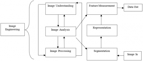
Depending on whether a pixel's intensity value is larger or lower than a predetermined threshold, the image is separated into white and black pixels. Three layers of image engineering are shown in Figure 1. The upper layer is used for image understanding, the middle layer is used for image analysis, and the bottom layer is used for image processing. The result of image segmentation is significantly influenced by the precision of feature measurement. As image segmentation is a computer-aided process, the automation of segmentation is essential for medical imaging applications. The image segmentation and image engineering application areas are depicted in Figure 1.
Figure 1. Image engineering and image segmentation
3.3 FCM algorithm
The fuzzy clustering and hard clustering are two clustering strategies. Usually, just one cluster is assigned to each data point using hard clustering techniques. As a result, every pixel in an image belongs to one cluster, yielding extremely accurate results in image clustering. The effectiveness of hard clustering algorithms is diminished by several factors, including the intensity of homogeneities, the lack of contrast, the insufficient spatial resolution, overlap, and noise. The fuzzy clustering technique has been extensively researched and used to the process of image clustering and segmentation. It is a soft segmentation approach because it can withstand ambiguity and maintain more information than hard segmentation techniques. The FCM approach is used more often than other fuzzy clustering algorithms. This is among the reasons why it is so popular. For determining the optimal division, iterative FCM clustering is used to minimize the weighted within-group sum-of-squared error objective function.
$K_p=\sum_{a=1}^M \sum_{b=1}^N u_{a b}^p d^2\left(Y_a, V_b\right)$ (1)
where, $Y=\left\{Y_1, Y_2, \ldots Y_M\right\} \subseteq I R^m$ data that is stored in m-dimensional vector space, M consists of the total amount of data pieces, d refers to the total number of clusters that $2 \leq d<M$, $u_{a b}$ is the extent to which one is a member of $Y_{a}$ in the $a^{t h}$ cluster, p the weighting exponent that is applied to each fuzzy membership status, $V_{b}$ is an example of the center of cluster prototype iteration (b), $d^2\left(Y_a, V_b\right)$ a measurement of the distance between two objects $Y_{a}$ and cluster center $V_{b}$. An answer to the problem of the object function $K_{p}$ attainable using an iterative procedure, which is carried out in the following manner:
(1) Values for d, p and $\epsilon$ are set.
(2) Initialize the Fuzzy partition matrix $U^{(0)}$.
(3) Set the Loop counter b as b=0.
(4) Compute the Cluster centers $V_b{ }^{(b)}$ with $U^{(b)}$ using Eq. (2):
$V_j^{(b)}=\frac{\sum_{i=1}^N\left(U_{j i}(b)\right) m x i}{\sum_{i=1}^N\left(U_{j i}(b)\right) m}$ (2)
(5) Compute the membership matrix suing Eq. (3):
$V_j^{(a+1)}=\frac{1}{\sum_{k=1}^c\left(\frac{d_{j i}}{d_{k i}}\right)^{\frac{2}{n+1}}}$ (3)
(6) If max $\left\{U^{(b)}-U^{(b+1)}\right\}<\epsilon$ then stop, otherwise, set $a=a+1$ and go to step 4.
Figure 2 presents a comparison of the clustering results obtained by the FCM after applying it to a synthetic test image.
(a)
(b)
Figure 2. (a) Noisy image; (b) FCM result
3.4 FLICM algorithm
One novel and trustworthy FCM framework developed in this paper is the Fuzzy Local Information C-Means (FLICM) method. Although the approaches discussed in the preceding section produced satisfactory results for image clustering, they do have certain shortcomings. They aren't strong enough to withstand noise and anomalies, particularly when the noise is unknown in advance, even if using local spatial information makes them more noise resistant. A key parameter, denoted as $\alpha$ (or $\lambda)$, is incorporated into their objective functions to strike a balance between the efficacy of image detail preservation and resistance to noise. Choosing it usually requires some trial and error or expertise. It is expected that the new component will possess several unique qualities:
$H_{n m}=\sum_{p \in M_m}^m \frac{1}{e_{m p+1}}\left(1-v_{n p}\right)^0\left\|Y_p-U_n\right\|^2$ (4)
where, the $m^{t h}$ local window center is denoted by the pixel, reference cluster is referred as n, $p^{t h}$ it is recommended that the pixel be included in the accumulation of neighbors falling into a window inside the system, the $m^{t h}$ pixel $\left(M_m\right)$, $d_{i j}$ represents as the spatial Euclidean distance between each pair of pixels i and j, $u_{k i}$ means the extent to which one is a member of the $p^{t h}$ pixel in the $n^{t h}$ cluster, O is the weighted exponent that is applied to each fuzzy membership, and $U_{n}$ is the model of the center of cluster that is developed. n is a significant role played by $H_{n m}$ the application of the method will also be shown in the part that comes after this one. By using the definition of $H_{n m}$ the FLICM clustering technique is described as a robust framework for image clustering that utilizes fuzzy convolutional neural networks. It includes information about the local spatial and intensity level into its objective function, which is expressed in terms of $J_{m}$ in below equation.
$J_m=\sum_{m=1}^M \sum_{n=1}^d u_{n n}^{\circ}\left\|Y_p-U_n\right\|^2+H_{n n}$ (5)
The two necessary conditions for $J_{m}$ to be at its local minimal extreme, with respect to $u_{n m}$ and $u_{m}$ is obtained as follows:
$u_{k i}=\frac{1}{\sum_{j=1}^c\left(\frac{\left\|X_i-V_k\right\|^2+G_{k i}}{\left\|X_i-V_j\right\|^2+G_{j i}}\right)\left(\frac{1}{m-1}\right)}$ (6)
$V_k=\frac{\sum_{i=1}^N u_{k i} m_{x i}}{\sum_{i=1}^N u_{k i} m}$ (7)
Thus, the FLICM algorithm is given as follows:
(1) Initialize the fuzzification parameter (m), cluster prototypes (c), and the stop condition $\epsilon$.
(2) Initialize the Fuzzy partition matrix.
(3) Initialize the Loop counter b as b=0.
(4) Compute c using Eq. (6).
(5) Compute the Membership values using Eq. (7).
(6) $\max _{i j}\left\{U^{(b)}-U^{(b+1)}\right\}<\epsilon$ then stop, otherwise, set b=b+1 and go to step 4.
Figure 3 shows the comparison of clustering results on synthetic test image by the FCM and FLICM techniques.
(a)
(b)
(c)
Figure 3. (a) Original image; (b) FCM Result; (c) FLICM Result
3.5 Proposed KWFLICM algorithm
The proposed KWFLICM algorithm enhances image segmentation by accurately detecting irregular shapes and boundaries of lung cancer tissues. This section shows how KWFLICM improves upon traditional clustering techniques like FCM and FLICM, especially in lung cancer detection. The challenges in lung cancer identification are as follows:
KWFLICM addresses these challenges by integrating kernel methods with spatial weighting, making it especially effective for lung cancer image segmentation. FCM lustering algorithm calculates a membership value for each pixel based solely on pixel intensity, which limits its ability to handle noise and fuzzy boundaries. FLICM incorporates spatial information from neighboring pixels to improve noise resilience, but it may still struggle with complex textures and irregular boundaries in lung images. KWFLICM improves upon these by using kernel functions and weighted local spatial information, enabling better differentiation of cancerous regions. The key enhancement in KWFLICM is the kernel function, which transforms data to a higher-dimensional space. This allows KWFLICM to:
KWFLICM uses a weighted local spatial information mechanism that considers both the intensity and spatial proximity of neighboring pixels. This helps in:
The KWFLICM algorithm optimizes an objective function that minimizes:
The KWFLICM algorithm follows these steps in lung cancer identification:
In lung cancer identification, KWFLICM's combination of kernel functions and weighted spatial information improves the algorithm’s ability to handle noise, detect complex boundaries, and capture small, irregular cancerous regions. This enhances the accuracy of segmentation, making KWFLICM a powerful tool for identifying and analyzing lung cancer in medical imaging. Kernel parameters are typically chosen in the KWFLICM algorithm for lung cancer identification: The choice of kernel function is as follows:
The RBF kernel parameter (σ) controls the smoothness of the Gaussian curve, influencing the radius of influence for each pixel’s similarity with neighboring pixels. The optimal values for σ are often found through cross-validation by comparing different values on a set of sample images, selecting the one that achieves the best segmentation accuracy. For lung cancer images, σ is usually chosen based on pixel intensity ranges and the image resolution, as lower σ values capture finer details, while higher σ values generalize more. The degree (d) in polynomial kernel controls the complexity of the polynomial surface. Higher degrees can capture more complex relationships but can also lead to overfitting. The coefficient (c) shifts the polynomial surface, controlling the sensitivity of the kernel function to pixel intensity differences. Typically, the values of d range from 2 to 4 ensure the polynomial function is neither too simple nor too complex for the lung images. The coefficients are manually adjusted based on visual inspection of segmentation results; high values may enhance contrast but also risk introducing artifacts.
The fuzzy clustering approach is the most essential clustering method for image segmentation since it can preserve more information about the image than the hard clustering method. The FCM approach is a popular fuzzy clustering method for image segmentation. Many considerations must be satisfied for a fuzzy clustering method to function as intended. Concerns about the initialization of the clustering method, cluster size and form, cluster distribution, cluster number in the data, and cluster number are at the heart of these problems:
$J_m=\sum_{k=1}^M \sum_{l=1}^N u_{k i} m\left\|Y_k-A_l\right\|^2, 1 \leq m<\infty$ (8)
where, $u_{i j}$ is the degree of membership of $Y_{k}$ in the cluster k, m is any real number larger than 1, the d-dimension center of the cluster is $A_{l}$, along with that $\left\|Y_k-A_l\right\|$ represents any norm that expresses the degree of similarity between a set of measured data and the center of the set and $i^{t h}$ of d-dimensional measured data is $Y_{k}$. The process of fuzzy partitioning may be carried out by performing an iterative optimization of the objective function that is provided before, with the status of membership being updated during the process. $u_{i j}$ and the cluster centers $A_{l}$ by:
$v_{k l}=\frac{1}{\sum_{p=1}^a\left(\frac{\left\|Y_k-A_l\right\|}{\left\|Y_k-A_p\right\|}\right)^{\frac{2}{n-1}}}$ (9)
$A_j=\frac{\sum_{i=1}^N u_{i j}^m x_i}{\sum_{i=1}^N u_{i j}^m}$ (10)
After $\max _{i j}\left\{\left|u_{i j}^{(k+1)}-u_{i j}^k\right|\right\}<\epsilon$, the iteration will stop, where, $\epsilon=[0,1]$ a termination criterion and the iteration steps are denoted by k. This process converges with a saddle point of $J_{m}$ or local minimum. When it comes to noise-free images, the FCM methods outperform more traditional algorithms. However, images contaminated with noise, outliers, and other imaging aberrations cannot be segmented using this method. FCM generates findings that are not robust for several reasons, the most significant of them are the use of a Euclidean distance and the absence of spatial contextual information in the image that is not robust. Many other FCM algorithms that have been improved have been offered in attempt to find a solution to the first difficulty. Each of these algorithms incorporates local geographical data into the FCM goal function that is first developed. Within the framework of the FCM_S algorithm, the spatial neighborhood term is included to bring about a modification to the mission function of FCM.
One of the most significant downsides of FCM_S is that the computation of the spatial neighborhood term requires a significant amount of time during each iteration step. This presents a significant challenge for the algorithm. It is decided to construct two distinct versions of FCM_S, namely FCM_S1 and FCM_S2, to lessen the amount of computing effort that is needed by FCM_S. To improve the overall performance of the model, the neighborhood term of FCM_S is changed to a median-filtered image in FCM_S2, while an additional mean-filtered image is included into FCM_S1 to further improve its performance.
The capacity to calculate the mean- and median-filtered images in advance results in a reduction in the operating expenses associated with processing. Enhanced FCM (EnFCM) is created for accelerating the process of image segmentation. For producing a linearly weighted sum image, it makes use of the original image as well as the average grey level of each pixel in the surrounding neighborhood. The combined image's grey level histogram is then used for categorization. The computational complexity of EnFCM is less. However, these methods do not allow for the direct application of the source image. To manage the balance between robustness against noise and detail preservation efficacy, they require certain parameters, denoted by an or λ. To address these issues and improve image segmentation performance, a new parameter-free robust FLICM is introduced. By defining a new fuzzy factor, FLICM supplants parameter a, which has been used by all prior methods and variations.
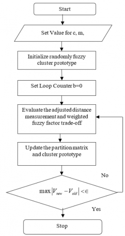
One of the objectives is to develop a trade-off WFF that is capable of being used for the purpose of adaptively controlling the local spatial connection. The distance that separates neighboring pixels and the difference in intensity levels between them are the two factors that define this section. To enhance the FLICM method, a trade-off WFF and kernel approach are employed. Both the intensity and the spatial distance between adjacent pixels are considered by the tradeoff WFF. Moreover, there are no parameters for the kernel distance measure, or the tradeoff WFF. Following segmentation using the FCM, FLICM, and KWFLICM algorithms, the tumor region from the segmented image is shown separately. Figure 4 displays the algorithm's flow chart.
Figure 4. Flow chart representation of KWFLICM algorithm
The following is a concise summary of the algorithm that has been proposed:
If $max \left|V_{ {new }}-V_{ {old }}\right|<\epsilon$ then stop, otherwise, set b = b+1 and go to step 4. $V=V_1, V_2, \ldots V_c$ are vectors that represent the prototypes of the clusters. After the algorithm has reached a point of convergence, the defuzzification procedure is carried out to provide a segmented image that is clear and distinct.
3.6 Membership function
Fuzzy sets' Membership Function (MF) is a simplified version of classical sets' indicator function. As an expansion of value, the MF in fuzzy logic stands for the degree of truth. Although they are conceptually different, degrees of truth and probabilities are sometimes used interchangeably. Fuzzy truth, on the other hand, denotes membership in nebulously defined sets rather than the probability of a certain occurrence or situation. A membership function for a fuzzy set A on the universe of discourse X is denoted as: X $\rightarrow$ [0,1], where each element of X is mapped to a value in between to 0 and 1.
3.6.1 Cluster prototype
Fuzzy modeling, data analysis, image processing, pattern recognition, and FCM algorithms are just a few of the applications that have made extensive use of fuzzy clustering approaches based on objective functions. Using fuzzy clustering techniques, it is feasible to ascertain an underlying structure that exists within the data. The data set is divided into groups that overlap with one another, which is one instance of these methodologies. To obtain better results, a technique that employs fuzzy clustering must consider a variety of distinct elements. The configuration of the clustering method, the number of clusters present in the data, the form and size of the clusters, and the distribution of the data pattern should all be taken into consideration. Computing the morphologies of the clusters is accomplished via the use of methods that combine point prototypes with the distance measure. Data points from linked clusters with membership 1.0 should be included in the cluster prototypes, which should also extend a certain distance from the cluster centers, according to this suggestion. This is not a characteristic of current clustering methods. The sensitivity of fuzzy clustering algorithms to initialization is well-known. It is common practice to randomly start the algorithms numerous times in the hope that one of them would yield a good clustering result. A very diverse distribution of data patterns makes the system more sensitive to startup.
3.6.2 Trade-Off weighted fuzzy factor
The noise resistance asset of the proposed KWFLICM mainly relies on the fuzzy factor $H_{m n}$ as shown in below equation.
$H_{m n}=\sum_{i=1}^N \sum_{k=1}^c u_{m n}^m \sum_{i \neq j}^N V_{a b}\left(1-V_{m n}\right)^m\left(1-J\left(Y_a, U_m\right)\right)$ (11)
To what extent the adaptive trade-off WFF considers local intensity-level and geographical constraints are context dependent. The spatial constraint is defined as the amount to which neighboring pixels with respect to spatial distance from the center pixel (in terms of both $p_{i}$ and $q_{i}$) dampen the effect of pixel $x_{i}$.
$W_{s c}=\frac{1}{d_{i j}+1}$ (12)
where, the $i^{t h}$ local window center is denoted by the pixel $N_{i}$ and the $j_{t h}$ pixel is a representation of the collection of neighbors that have fallen into the window surrounding it the $i^{t h}$ pixel, $d_{i j}$ refers to the Euclidean distance between the two points in space $j^{t h}$ the pixel at the center, as well as the neighboring particles. The impact of the pixels included inside the local window may change in a flexible way according to their distance from the center pixel because of the specification of the spatial component. This is because the local window is a locally contained area. Because of this, it is possible to make use of extra information that is in the immediate vicinity. Table 1 shows a 3×3 layout that depicts the window with noise as well as the dampening extent of the neighbors.
Table 1. Noise and the amount to which neighbors dampen it are shown in a 3×3 window (a) No noise in the central pixel; (b) Noisy pixels have ruined the center pixel; (c) The surrounding area's level of moisture
|
A90 |
22 |
13 |
87 |
99 |
116 |
0.414 |
0.5 |
0.414 |
|
2 |
20 |
35 |
90 |
20 |
67 |
0.5 |
|
0.5 |
|
28 |
B120 |
27 |
110 |
88 |
77 |
0.414 |
0.5 |
0.414 |
|
(a) |
(b) |
(c) |
||||||
An instance of this may be seen in Table 1(a), which shows a 3×3 window taken from the noise image, and Table 1(c) shows how its neighbors' damping extent varies with spatial distance. By including the fuzzy factor, Table 2 illustrates the changes in membership values corresponding to Table 1(a). Table 2 shows that when the iteration counts get up, the membership values of noisy and no-noisy pixels converge on a common value, and the noisy pixels are ignored. The method converges after five rounds. In this scenario, the intensity level values of the noisy pixels are distinct from those of the other pixels included inside the window, while the fuzzy component contributes to the overall pattern ($G_{k i}$) balances their own membership values. Every single pixel that is included inside the window is a member of the same cluster. Accordingly, the factor incorporates both the intensity level and the spatial limitations, which together form the combination $G_{k i}$, the impact of the noisy pixels should be suppressed.
Table 2. Membership values (a) Initial membership values; (b) After a single phase; (c) Subsequent to two iterations; (d) three times through the process; (e) Subsequent to four iterations; (f) Similar membership values
|
0.576 |
0.477 |
0.962 |
0.782 |
0.877 |
0.926 |
0.877 |
0.997 |
0.949 |
|
0.626 |
0.242 |
0.736 |
0.923 |
0.842 |
0.963 |
0.969 |
0.981 |
0.984 |
|
0.626 |
0.496 |
0.710 |
0.896 |
0.776 |
0.970 |
0.985 |
0.837 |
0.982 |
|
V1=50, V2=100 |
V1=32, V2=128 |
V1=28, V2=126 |
||||||
|
(a) |
(b) |
(c) |
||||||
|
0.881 |
0.994 |
0.972 |
0.882 |
0.992 |
0.981 |
0.882 |
0.992 |
0.982 |
|
0.962 |
0.992 |
0.984 |
0.954 |
0.996 |
0.989 |
0.954 |
0.996 |
0.989 |
|
0.979 |
0.852 |
0.996 |
0.973 |
0.865 |
0.998 |
0.972 |
0.865 |
0.998 |
|
V1=26, V2=122 |
V1=21, V2=119 |
V1=19, V2=120 |
||||||
|
(d) |
(e) |
(f) |
||||||
The element $G_{k i}$ is also decided automatically rather than being set synthetically. It does not know any information about the noise. Hence, the algorithm becomes more resistant to the outliers being used. Following that, the coefficient of variation at the local level $C_{j}$ for each pixel j as $C_j=\frac{{var}(x)}{x^2}$ is obtained. $C_{j}$ displays how consistent the intensityscale of the window that is around it is. Because of this, the values are low in regions, while the values are high at edges or in locations where there is noise corruption. According to the data point distance variance, the degree of aggregation that exists around the clusters may be determined. Although there is just a little amount of variance, the clusters are somewhat near to one another and are spread out around their cores. To restate, it is envisaged that membership will be shown separately if the dataset contains recognizable clusters. Members will be exhibited individually.
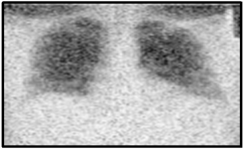
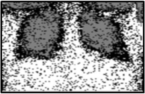
The ELCAP [23] and LIDC benchmark datasets [24, 25] are used to assess how well the suggested method performs in lung nodule identification. The DIOCOM format is used to store lung CT images, and each scan has 512 pixels in width and 512 pixels in height. Figure 5 displays the image of a human lung with a tumor that is used as the input image. The input image is clustered using the FCM technique and then the clustered output is segmented into the tumor region using the histogram approach. The FCM algorithm takes less time to execute than the FLICM and KWFLICM algorithms, but it is unable to cluster images with outliers or noise like salt and pepper. The FCM clustering and segmentation image is displayed in Figure 6. Given an input image, the FLICM algorithm is utilized to do the clustering. The tumor zone is divided from the FLICM algorithm's clustered output using the histogram approach. While the FLICM approach takes longer to execute than the other two, it produces better clustering results when compared to FCM in cases where the image contains outliers or salt and pepper noise. Figure 7 shows the FLICM segmentation and clustering image.
Figure 5. Input image
(a)
(b)
Figure 6. (a) FCM clustering image; (b) segmented image
(a)
(b)
Figure 7. (a) FLICM output; (b) segmented image
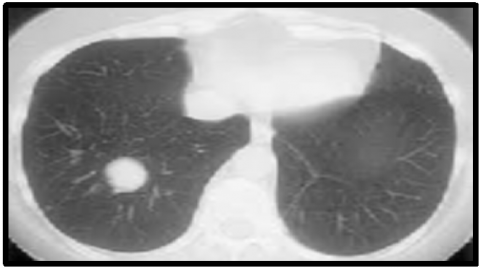
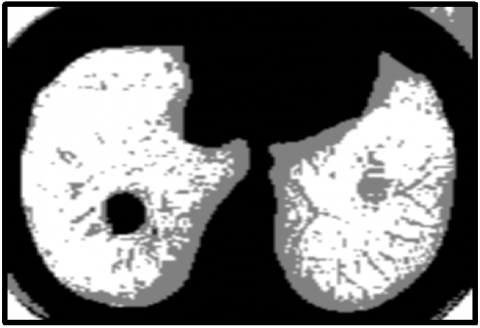
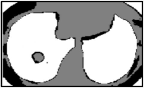
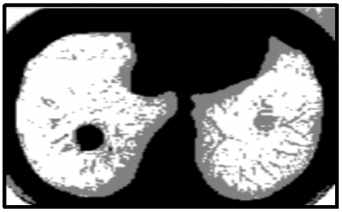
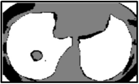
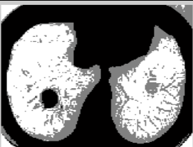
For clustering the input image, the KWFLICM algorithm is applied. After that, the tumor region is separated from the clustered output of the KWFLICM method using the histogram approach. When it comes to clustering results, the KWFLICM method performs faster than other FLICM algorithms and produces superior results when images contain outliers or salt and pepper noise. The KWFLICM segmentation and clustering image is displayed in Figure 8.
(a)
(b)
Figure 8. (a) KWFLICM clustered image; (b) segmented image
The KWFLICM algorithm has shown promising results in lung cancer identification, particularly in segmenting and detecting cancerous nodules from CT images. The findings from studies applying KWFLICM to lung cancer detection reveal several advantages over traditional algorithms, especially in handling the challenges of lung image data, such as noise, irregular shapes, and low contrast. Here's an overview of these key findings:
(1) Improved Segmentation Accuracy
Fine Boundary Detection: KWFLICM’s Kernelized approach enables it to better capture the fuzzy boundaries typical of lung cancer nodules. This allows it to differentiate between cancerous and non-cancerous tissues more accurately than traditional FCM and FLICM techniques.
Enhanced Shape Sensitivity: Lung nodules can have irregular shapes and textures, especially in early-stage cancers. KWFLICM's kernel transformation helps to detect these irregular shapes, leading to improved segmentation of nodules with complex, non-spherical boundaries.
(2) Noise Robustness
Weighted Local Information: The integration of spatial weights in KWFLICM enhances its resistance to noise, which is especially beneficial for low-dose CT images that can have low contrast and higher noise levels. This allows the algorithm to differentiate real nodule structures from image noise, crucial for accurate identification in low-quality scans.
Smoothing of Image Artifacts: KWFLICM's weighted approach also reduces the impact of artifacts often found in CT images, minimizing false positives from these artifacts and resulting in a cleaner segmentation output.
(3) Enhanced Detection of Small and Subtle Nodules
Sensitivity to Small Nodules: The kernel function in KWFLICM allows for mapping pixel intensity into a higher-dimensional space, which makes the detection of small, low-intensity nodules more effective. This is important for early lung cancer detection, where nodules may be tiny and less distinct.
Identification of Ground-Glass Opacities: Lung cancer is often presented as part-solid or ground-glass nodules, which can be challenging to detect with conventional methods. KWFLICM's ability to capture subtle pixel variations makes it better at identifying these less opaque nodules, a key feature for early diagnosis.
Table 3. Results comparison of FCM, FLICM and KWFLICM
|
Parameters |
FCM |
FLICM |
KWFLICM |
|
Input |
|||
|
Function |
Euclidean distance between pixels is used to perform clustering |
The local spatial information is used |
The local spatial information and kernel metric is used |
|
Clustering Output |
|||
|
Noise Tolerance |
Could not segment image with salt and pepper noise or outlier |
Provide better results compared with FCM |
Provide complete tolerance towards salt and pepper noise as well as outliers |
|
Segmentation Result |
|||
|
SD |
18.7697 |
19.6324 |
20.9823 |
|
Elapsed Time |
4.2576 |
28.7979 |
19.4958 |
|
Accuracy |
87.24 |
88.12 |
90.76 |
A comparison of the suggested system with the FCM and FLICM techniques is presented in Table 3.
(4) Reduced false positives
Improved Specificity: Due to noise and ambiguity in CT images, traditional FCM and even FLICM often have a higher false positive rate. KWFLICM reduces false positives by using kernelized fuzzy clustering, which can better distinguish between lung nodules and other lung structures (like blood vessels or non-cancerous nodules).
Efficient Noise Discrimination: By accounting for local spatial information and applying kernel functions, KWFLICM improves its ability to distinguish noise and artifacts from actual lung structures, further minimizing false detections.
(5) Scalability and Computational Efficiency
Fast Convergence: KWFLICM's implementation has been observed to converge faster than standard FCM and FLICM, particularly due to the influence of kernel functions that streamline the clustering process. This makes it feasible for real-time diagnostic applications.
Adaptive Parameter Tuning: The kernel parameters in KWFLICM can be fine-tuned to different datasets, enabling the algorithm to adapt to varying image quality or resolution, which is often encountered across different CT scanners or patient profiles.
(6) Comparison to Other Methods
Superior to FCM and FLICM: Studies comparing KWFLICM to FCM and FLICM show that KWFLICM achieves higher accuracy and sensitivity in detecting cancerous nodules, especially in cases with low contrast or noisy backgrounds. It is particularly effective in identifying challenging different nodule types in the LIDC and ELCAP databases.
Comparable with Advanced Machine Learning Models: In some cases, KWFLICM's performance is competitive with machine learning approaches, especially in terms of nodule segmentation accuracy. While it may not match DL methods in complex classification tasks, KWFLICM offers a simpler, interpretable approach with strong performance in segmentation.
KWFLICM demonstrates several critical advantages in lung cancer identification:
These findings highlight KWFLICM as a robust option for early-stage lung cancer identification and segmentation, particularly in cases where image quality and noise pose significant challenges.
The kernel approach has been used to address the problem of unsupervised clustering. Through the development of an unsupervised FCM technique that is based on a kernel metric, which is intended to segment images contaminated by noise and intensity in homogeneities. It has been proved that the combination of KDM and WFF is an efficient approach for constructing a trustworthy image clustering method. A trade-off between the amount of noise and the amount of image information can be established by the KWFLICM algorithm as it included a reformulated spatial constraint, and a trade-off WFF as a local similarity metric. Furthermore, the unique trade-off weight is mostly determined by the spatial limitations in the local area and the distribution of local information. This, in turn, influences the damping extent of pixels next to one another.
It is possible that it now includes local facts or information with more precision than it did in its previous iterations. In addition, the KDM and the trade-off WFF are fully independent of the computation of the parameters that have been altered via experimentation, enabling automated applications. The suggested algorithm's experimental result on an experimental image demonstrates how much it enhances image segmentation performance and robustness against various types of noise. The tumor region is then divided into discrete sections using the histogram approach. In comparison to previous segmentation techniques like FCM and FLICM, the KWFLICM method yields more reliable results for the identification of lung cancer. If some extra features are included, it can identify lung tumors more quickly and accurately and the kernel metric algorithm is modified. Simultaneously, techniques must be examined to illustrate the long-term consequences of the specific defects associated with the disease. The future work for KWFLICM in lung cancer identification encompasses a multifaceted approach that includes:
These strategies aim to enhance KWFLICM’s capabilities, making it a powerful tool for improving lung cancer detection and enhancing patient care.
[1] Venkatesan, P. (2019). Image fusion-Based lung nodule detection using structural similarity and max rule. International Journal of Advances in Signal and Image Sciences, 5(1): 29-35. https://doi.org/10.29284/ijasis.5.1.2019.29-35
[2] Naseer, I., Akram, S., Masood, T., Rashid, M., Jaffar, A. (2023). Lung cancer classification using modified U-Net based lobe segmentation and nodule detection. IEEE Access, 11: 60279-60291. https://doi.org/10.1109/ACCESS.2023.3285821
[3] Nejad, R.R., Hooshmand, S. (2023). HViT4Lung: Hybrid vision transformers augmented by transfer learning to enhance lung cancer diagnosis. In 2023 5th International Conference on Bio-Engineering for Smart Technologies (BioSMART), Paris, France, pp. 1-7. https://doi.org/10.1109/BioSMART58455.2023.10162074
[4] Jaya, V.J.M., Krishnakumar, S. (2024). Multi-classification approach for lung nodule detection and classification with proposed texture feature in X-ray images. Multimedia Tools and Applications, 83(2): 3497-3524. https://doi.org/10.1007/s11042-023-15281-5
[5] Shamas, S., Panda, S.N., Sharma, I. (2022). Review on lung nodule segmentation-Based lung cancer classification using machine learning approaches. In Artificial Intelligence on Medical Data: Proceedings of International Symposium, ISCMM 2021, Singapore, pp. 277-286. https://doi.org/10.1007/978-981-19-0151-5_24
[6] Aziz, K.A.A., Saripan, M.I., Saad, F.F.A., Abdullah, R.S.A.R., Waeleh, N. (2022). A Markov random field approach for CT image lung classification using image processing. Radiation Physics and Chemistry, 200: 110440. https://doi.org/10.1016/j.radphyschem.2022.110440
[7] Nageswaran, S., Arunkumar, G., Bisht, A.K., Mewada, S., Kumar, J.S., Jawarneh, M., Asenso, E. (2022). [Retracted] Lung cancer classification and prediction using machine learning and image processing. BioMed Research International, 2022(1): 1755460. https://doi.org/10.1155/2022/1755460
[8] Kasinathan, G., Jayakumar, S. (2022). Cloud‐based lung tumor detection and stage classification using deep learning techniques. Biomed Research International, 2022(1): 4185835. https://doi.org/10.1155/2022/4185835
[9] Said, Y., Alsheikhy, A.A., Shawly, T., Lahza, H. (2023). Medical images segmentation for lung cancer diagnosis based on deep learning architectures. Diagnostics, 13(3): 546. https://doi.org/10.3390/diagnostics13030546
[10] Salama, W.M., Aly, M.H. (2022). Framework for COVID-19 segmentation and classification based on deep learning of computed tomography lung images. Journal of Electronic Science and Technology, 20(3): 100161. https://doi.org/10.1016/j.jnlest.2022.100161
[11] Vinod, C., Menaka, D. (2022). Multimodal data analysis using soft computing techniques for the detection and classification of lung cancer. In 2022 Third International Conference on Intelligent Computing Instrumentation and Control Technologies (ICICICT), Kannur, India, pp. 150-153. https://doi.org/10.1109/ICICICT54557.2022.9917865
[12] Lavanya, M., Kannan, P.M., Arivalagan, M. (2021). Lung cancer diagnosis and staging using firefly algorithm fuzzy C-Means segmentation and support vector machine classification of lung nodules. International Journal of Biomedical Engineering and Technology, 37(2): 185-200. https://doi.org/10.1504/IJBET.2021.119504
[13] Meraj, T., Rauf, H.T., Zahoor, S., Hassan, A., Lali, M.I., Ali, L., Bukhari, S.A.C., Shoaib, U. (2021). Lung nodules detection using semantic segmentation and classification with optimal features. Neural Computing and Applications, 33: 10737-10750. https://doi.org/10.1007/s00521-020-04870-2
[14] Wang, J., Wang, J., Wen, Y., Lu, H., Niu, T., Pan, J., Qian, D. (2019). Pulmonary nodule detection in volumetric chest CT scans using CNNs-based nodule-size-Adaptive detection and classification. IEEE Access, 7: 46033-46044. https://doi.org/10.1109/ACCESS.2019.2908195
[15] Li, Z., Li, L. (2017). A novel method for lung masses detection and location based on deep learning. In 2017 IEEE International Conference on Bioinformatics and Biomedicine (BIBM), Kansas City, MO, USA, pp. 963-969. https://doi.org/10.1109/BIBM.2017.8217787
[16] Rahman, M.S., Shill, P.C., Homayra, Z. (2019). A new method for lung nodule detection using deep neural networks for CT images. In 2019 International Conference on Electrical, Computer and Communication Engineering (ECCE), Cox'sBazar, Bangladesh, pp. 1-6. https://doi.org/10.1109/ECACE.2019.8679439
[17] Zuo, W., Zhou, F., Li, Z., Wang, L. (2019). Multi-Resolution CNN and knowledge transfer for candidate classification in lung nodule detection. IEEE Access, 7: 32510-32521. https://doi.org/10.1109/ACCESS.2019.2903587
[18] Cao, H., Liu, H., Song, E., Ma, G., Xu, X., Jin, R., Hung, C.C. (2019). Multi-branch ensemble learning architecture based on 3D CNN for false positive reduction in lung nodule detection. IEEE Access, 7: 67380-67391. https://doi.org/10.1109/ACCESS.2019.2906116
[19] Günaydin, Ö., Günay, M., Şengel, Ö. (2019). Comparison of lung cancer detection algorithms. In 2019 Scientific Meeting on Electrical-Electronics & Biomedical Engineering and Computer Science (EBBT), Istanbul, Turkey, pp. 1-4. https://doi.org/10.1109/EBBT.2019.8741826
[20] Rao, A., Chu, S., Batlivala, N., Zetumer, S., Roy, S. (2018). Improved detection of lung fluid with standardized acoustic stimulation of the chest. IEEE Journal of Translational Engineering in Health and Medicine, 6: 1-7. https://doi.org/10.1109/JTEHM.2018.2863366
[21] Mukherjee, M., Biswal, P.K. (2018). Segmentation of lungs nodules by iterative thresholding method and classification with Reduced Features. In 2018 Second International Conference on Inventive Communication and Computational Technologies (ICICCT), Coimbatore, India, pp. 450-455. https://doi.org/10.1109/ICICCT.2018.8473287
[22] Li, L., Wu, Y., Yang, Y., Li, L., Wu, B. (2018). A new strategy to detect lung cancer on CT images. In 2018 IEEE 3rd International Conference on Image, Vision and Computing (ICIVC), Chongqing, China, pp. 716-722. https://doi.org/10.1109/ICIVC.2018.8492820
[23] ELCAP Public Lung Image Database. (2003). http://www.via.cornell.edu/databases/lungdb.html.
[24] Armato, S.G., McLennan, G., Bidaut, L., McNitt‐Gray, M.F., et al. (2011). The lung image database consortium (LIDC) and image database resource initiative (IDRI): A completed reference database of lung nodules on CT scans. Medical Physics, 38(2): 915-931. https://doi.org/10.1118/1.3528204
[25] Armato, S.G., McLennan, G., Bidaut, L., McNitt-Gray, M.F., et al. (2015). LIDC-IDRI. The Cancer Imaging Archive. https://doi.org/10.7937/K9/TCIA.2015.LO9QL9SX