Machine Learning-Based Classification of Mosquito Wing Beats Using Mel Spectrogram Images and Ensemble Modeling

Nowadays, fever is a common disease spreading globally. The main root cause of fever spread is mosquitoes [1]. Various kinds of fevers are spreading and infecting people through different types of mosquitoes. According to a 2019 report by the World Health Organization (WHO), almost 400,000 deaths were caused by malarial fever alone [2]. Particularly in India, deaths due to dengue fever are 17,546 per 100,000 people. Fevers, when they turn into serious infections, may lead to different life-threatening complications such as chikungunya, dengue, Zika, and yellow fever [3].

The main aim is to detect mosquito wing beat sounds during flight in an acoustic time series. The key scientific modules that support this work provide the necessary data for the development of machine learning models to identify and classify occurrences in the dataset. The outcomes obtained from this audio detection are generated, examined, and applied to the audio information gathered in the field [4].

Traditional examination approaches for malaria, such as recording mosquitoes landing on human surfaces, consume more time, space, and money. The research also addresses the complications of disease contraction, which are critical for elimination efforts [5]. Due to these challenges, many vector methods representing the geographical spread of these insects rely on sparse, unevenly divided bi-directional data [6].

However, the models used in this work are concerned with one such processing region, which faces typical risks such as data imbalance, inadequate information, low transmission rates, selection bias, and varying labels. Therefore, this study considers other contexts and broader detection conditions, such as acoustic time series information [7].

The aim of this work is to develop a proper mechanism to detect the type of mosquito based on the breed that spreads malaria, using their wing beat features [8]. By doing so, we can implement the necessary structure to aid malaria-infected areas where it is needed the most. Additionally, these models can enhance audio machine learning algorithms. These enhancements are crucial in the study of feature extraction, using deep learning methods to work with widely available yet imperfectly labelled data [9, 10].

This work necessitates an essential automatic information system for detecting and classifying various mosquito species to aid in targeting the crucial areas affected by disease spread [11, 12]. With the help of these technologies, health organizations and other stakeholder groups can effectively identify disease-spreading mosquitoes and focus on infection hotspots [13, 14]. By understanding the dangerous threats and the increase in infections, the implemented techniques successfully help epidemiologists enhance scientific conclusions and methodologies [15]. Officials can be notified to take preventive measures in controlling the spread of infections by following specific steps in the infected regions [16, 17]. In this research, a hybrid machine learning algorithm is proposed for classifying mosquito species based on their wing beat sounds.

To detect the stream of audio, the algorithm, with the help of machine learning, is implemented in a three-step succession. The components are used to extract the audio signal data for a required time period. This data is then converted into necessary frequency components such as frequency and amplitude [18]. The spectral form is generally used as input to the network for noise identification. The type of spectroscopic format utilized significantly affects the efficiency of the network methods. Classifiers trained through this method represent human perception due to the Mel Frequency Cepstral Coefficient (MFCC), which gathers data at shorter wavelengths that are recognizable to humans [19, 20]. Consequently, the MFCC is widely used in this study as a primary spatial frequency factor. The workflow through machine learning to classify mosquito types based on the wing beat audio file is represented in Figure 1.

1.png

Figure 1. Work flow of ML for classification

In this research, we also considered the functioning of MFCC to feed data into the classifier. The extraction of features converts the MFCC data into a feature format for the audio signal to detect the signalling class. Obtaining the average vector values of spectral information is a standard phase in characteristic selection models.

The main objectives of this work are divided into following stages:

a) Firstly, the sound of a wingbeats is transformed into wave forms through black and white channels (binary) from the raw audio data.

b) The Mel spectrogram is used to remove the embedded noise which is required in maintaining the frequency formats of RGB image.

c) This modified image is now sent to CNN architecture for retrieving the embedded features with the help of convolutions.

d) Through fully connected layer, the final vector values are obtained and are given to ML classifiers for classifying the intensity of wingbeats of mosquitoes depending upon their range of frequencies.

The remaining sections of this is framed as: Section-2 discusses about ‘Related Works’, Section-3 discusses about ‘Methodology’, section-4 for describing ‘Results and its discussions and section-5 for ‘Conclusion with link to Future Scope’.

3.1 Dataset

In this study, data is used from the Kaggle repository [32]. This dataset contains information related to different varieties of mosquitoes along with their wing beat sounds. It includes 279,566 recordings of wing beats pertaining to six mosquito species: Aedes aegypti, Aedes albopictus, Anopheles arabiensis, Anopheles gambiae, Culex pipiens, and Culex.

The proposed model used in this work employs a group of informational techniques to ensure that the evaluated results meet a high standard of accuracy. Additionally, it is designed to identify different methods to process audio format data with minimal computational effort. The feature extraction model developed in this study plays a crucial role in classification, selecting the required and necessary traits. A sample summary of the information used in this research work is shown in Table 1.

Table 1. Summary of mosquito wing beat recordings [31]

3.2 Analysis of audio data

Audio signals are represented through sound waves, which can propagate through various transmission media such as gas, liquid, or as ultrasonic waves. In terms of magnitude and time, these signals typically remain constant. They can be quantized in two dimensions to be arranged digitally as time-series data.

A time series is defined as a sequence of data points labeled by time, making it a group of random values. The theoretical approach involves a constant alignment of information with exponential factors such as mean and variance, which may vary depending on the time interval. The samples are quantized to their nearest values within the group of digital ranges. This process of digital transmission speed is commonly grouped as periodic and associated. The accurate conversion of spectrum signals at a certain sampling frequency is twice the resonance value of relevance, referred to as sampling. During the encoding process, the calculation of amplitude generates intermittent values.

The final outcomes of raw frequencies are extracted and transformed into a waveform in WAV format, as shown in Figure 2. Ranging from 440 Hz to 5.1 KHz, the sound wave in WAV format of a mosquito over 5 seconds is represented in Figure 3. The image factors in the audio and every change in the waveform are explained in the sections below with the help of the mentioned figures.

2.png

Figure 2. Wave form in WAV of mosquito wing beats

3.png

Figure 3. Mel spectrograms of mosquito wing beats

Intermediate methods are commonly deployed through electronic sound waves. These methods are utilized as data in the evaluation of acoustic factors. Generally, these representations accurately record how humans recognize audio signals by altering the division of frequencies over time. They rely on both low- and high-level acoustic estimations, as well as musical presentations, and thus mid-level features have their specific term.

The intermediate concepts broadly used in the study are frequency and time. These constitute the amplitude and energy required for transmission at different frequencies. Frequencies vary over time along a wider timeline, and they perform transmission as the magnitude also changes. These predictions, in reality, act as a substitute for frequency in terms of accuracy with time resolution.

The commonly used time-frequency forms are developed using a spectrum analyser. The execution of a Short Time Wavelet Transformation (STWT) with initial frames attempts to stabilize and generate a waveform using Fourier Transform (FT). The energy in various bandwidths among the transformed frames is initiated through electric spectra, which are combined to develop a single frame. The derived characteristics are produced by converting the resulting image into a vector form. Generally, a Fourier Transform is considered the exceptional transformation from which most intermediate forms are derived. This is shown in Eq. (1) to brief the STFT along with some perceptions.

$F T\{x(t)\}=\int_{-\infty}^{+\infty} x(t) e^{-i w t} d t$       (1)

The functioning of a frame that is positive for a particular period of time consists of a variable that needs to be transformed, x(t). Considering the Fourier Transform of the complete signal under a single frame, it is progressed with a time vector to produce a two-dimensional representation of the data. For enhancing the characteristic features during the post- processing phase, the spectrograms are significantly modified. To show the corresponding volumes at different frequencies, the wavelengths present in the spectrum analyser are converted to a logarithmic scale.

Generally, a randomly selected variable is chosen for time-series data. This is done among samples that are close in time, making them more likely to be connected, compared to those that are farther apart. Additionally, time-series methods are utilized in chronological pairing, where the allotted time value has some connection with previous data, rather than with isolated values.

A signal is defined as data that represent compulsive phenomena. The audio channel utilized in the study is represented as a sample of metadata. The main aim of the study is to extract signals from audio data, which typically contain a significant amount of noise. Since noise is present in almost all real-world fields, it is important for machine learning to have the capability to recognize and address this concept.

Noise is referred to as any unreliable or unconnected data present in the evaluation. Noise is typically produced due to obstructions during the recording process. In simple terms, noise is a factor that introduces irregularity in the digital signal. It does not contain any information regarding the crucial variables used in the study. The correlation function value $R_s(T)$ is the power of a signal $s(t)$ when it in imaginary process that is constant is defined in Eq. (2):

$R_s(T)= Expected\,\,Value (s(t) * s(t+T))$       (2)

Related connections are managed between its correlation function and the power of noise $P_n$   is represented in Eq. (3):

$P_n= Expected\,\,Value \left(n^2(t)\right)$             (3)

3.3 Proposed model

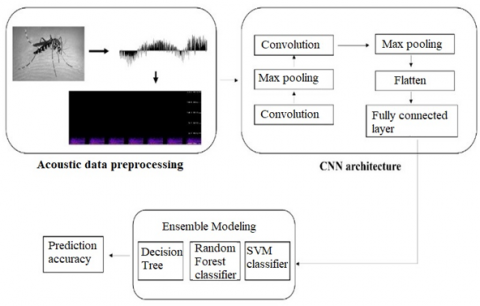
Our proposed model is illustrated in the workflow by organizing different kinds of mosquitoes based on the sound of their wing beats, as shown in Figure 4. The methodology is divided into three sections: Firstly, the pre-processing phase where the raw audio is processed; and finally, with the help of classifiers like RF (Random Forest), SVM (Support Vector Machine), DF (Decision Forest), and CNN (Convolutional Neural Network), the spectrogram images are processed.

During the pre-processing phase, the raw audio data is given as input to identify the intensity of the mosquito wing beat audio. All the intensities obtained from different audio files are grouped to develop a waveform in WAV format. There may be a chance of missing frequencies due to background noise. To eliminate this noise, Mel spectrogram filters are utilized to maintain the quality of the audio data. After this, the smooth waveform obtained is converted to spectrograms by producing a re-sampled frequency with a range of 440 Hz to 5.1 KHz.

In the second phase, the raw image format file is given as input to the CNN technique for feature extraction. Convolutions are developed during the encoding process. They are utilized in the CNN methodology to reduce the spectrogram image size. To minimize the number of shift values in a hidden layer, a batch normalization layer is added for each pooling and convolutional pair. This helps to increase the learning speed and reduce overfitting. Once the pooling process is completed, a layer called the flatten layer is produced. To further reduce overfitting, the flatten layer maintains a dropout rate of 50%. The final layer, called the fully connected layer, integrates an activation process, making it robust.

In the final phase, the established features from the CNN architecture are given to classifiers as input. The classifiers SVM, DT, and RF are used in the methodology to classify the sound of the mosquito. An ensemble model is used in this phase along with the classifiers. Based on the outcome of each classifier, the accuracy is detected and the recorded sound of the mosquito wing beat is identified.

4.png

Figure 4. Proposed methodology

3.4 Decision tree (DT)

In a decision tree (DT), the non-leaf nodes represent quality checks on the applied factors, each branch shows the outcome of the given input, and every terminal node includes a classifier. The main root of the decision tree is the node located at the top of the tree structure. The decision tree is formed by dividing the dataset, which acts as the structure of the tree. The primary reason for this division is the collection of various feature nodes based on classification features. For every developed subset in the tree, recursive partitioning is performed. The Gini Index can be calculated, by considering the probability P_i of the chosen node having the label i along with the classification error for that node ‘ $\sum_{k \neq i} P_k$’. This becomes zero when every sample in the node support within a single region. Let us suppose P_i is proportion of the nodes in a given group of k items in the same class with i label which is given by Eq. (4):

$Gini\,\,Index=\sum_{i=1}^k P_i \sum_{K \neq i} P_k$            (4)

A disadvantage of conventional methods in implementing decision trees is that when the branches of the tree have deep roots, they may extend to overfitting the corresponding training data, resulting in limited bias but increased variance. To diminish this variation, the Random Forest algorithm groups multiple hierarchical decision trees constructed on different portions of the same dataset. This technique helps enhance the accuracy of our developed model. However, the total cost of the model sees a slight rise in bias and also experiences a slight decrease in accuracy.

3.5 Random Forest (RF)

The commonly used model of resampling, also known as bootstrapping, is employed in the Random Forest model for identification. This prediction method in the classifier is used to build the decision trees. Bootstrapping constantly among the randomly selected by restoring the test phase through a training dataset set $X=\left\{X_1, X_2, X_3, \ldots X_n\right\}$ with solutions $Y=\left\{Y_1, Y_2, Y_3, \ldots Y_n\right\}$ develop a tree for all the selection. The training variables ‘X_b’ and ‘Y_b’ are relied on a classification tree. Gathering the highest count of votes from every individual classification method on sampling after training, identification for unknown data X can is evolved.

The bootstrapping model decreases the variance without affecting the bias. If the bias remains unchanged, the model works efficiently. Consequently, single tree detection is accurate in the training dataset. The mean of various other trees is calculated when the trees are irrelevant. By using different training datasets for trees, the random sampling model interlinks the nodes, which results from training a number of trees in a single phase of training.

3.6 Support vector machine (SVM)

The SVM, also known as a quadratic classifier, shows an ideal representation by having a higher dimensional space among the subclasses. The basic functions represent the maximum distance between the regions and the hyperplane. Tolerance is allowed for a few misclassifications that are out of range, evaluated under the border range of the SVM classifier. The SVM classifier is related to kernel models that encompass a wide class of methodologies, which use kernel methods to transform features into a high-dimensional training dataset. Consequently, a hyperplane is plotted along the entire process of the training dataset. The classifier has unpredictable division rules. Considering the binary classification problem under the construction of linear methods is represented in Eq. (5).

$y(x)=W^T \emptyset(X)+b$            (5)

We have the final biased parameter ‘ $b$’ and represented ‘ $\emptyset(X)$’ as a translation of feature extractor. Keen observation has to be done so that the dual method eliminates working in feature set directly and is outlined in terms of basic functions.

The input vectors $x_1, x_2, x_3, \ldots x_n$ with matching detected values $t_1, t_2, t_3, \ldots t_n$ build the initial sample, and new data points $x$ are detected relying on the indication of $y(x)$. Since the trained model is differentiable in higher dimensional space, there must have at least one combination of the specifications w and b that allows a component of Eq. (6) to satisfy $y\left(x_n\right)>0$ for observations with $t_n=+1$ and $y\left(x_n\right)<0$ for points with $t_n=-1$, resulting in $t_n y\left(x_n\right)>0$ for all training samples.

The border range is calculated as the shortest distance between the decision function and each observation. This is how the SVM addresses this problem. In SVMs, the margin-maximized decision function is chosen as the classifier, as given by Eq. (6).

$t_n\left(W^T \emptyset\left(X_n\right)+b \geq 1\right.$, $where\,\,n=1, \ldots, N$           (6)

3.7 Convolutional neural network (CNN)

Every phase in a feed-forward deep network comprises a set of neurons. These neurons evaluate a non-linear element. This evaluation of the input layer is done after finding the linear combination of weights, $z=W^T X+b$. Thus, the parameters of the deep network method, using weights and biases, are developed. The group of sigmoid functions that contain the logistic function is a common choice for the activation function, as represented in Eq. (7).

$\sigma(z)=\frac{1}{1+e^{-z}}$              (7)

A fully connected network with at least one convolutional layer is defined as a Convolutional Neural Network (CNN). CNNs use convolutions instead of ordinary complex numbers during the process. They are primarily used to represent hierarchical methods, such as the grid organization of pixel intensities or commonly processed streams of audio. CNNs are useful in combining neighbouring spatial data in every medium. They contain convolution and pooling layers with fixed interconnections. The process of convolution generates a stack of extracted characteristic mappings. The input layers of the characteristic space are grouped together using convolution filters. To achieve efficiency, the number is substituted in the group of these convolutional layers using a complex number $W^l a^{(l-1)}$. The output of the signal, having at least one feature map $a^l$ is shown mathematically in Eq. (8) as a set, where the convolution filters are denoted by W and the feature map is denoted by $a^{(l-1)}$.

$a^l=\sigma\left(b+W^l a^{l-1}\right)$             (8)

The execution of a neural network through convolution is represented in Figure 5. It is parameterized to detect two classes from a three-channel image (RGB) with a size of 32×32. The outcome of the convolution having filtering process denoted by W is shown in Eq. (9) for every j and $k^{t h}$ neurons located in the hidden layer of the classifier.

$\sigma\left(b+\sum_{l=1}^n \sum_{m=1}^n w_{l, m} a_j+l, k+m\right)$            (9)

where, $a_{x, y}$ represents the input activator at certain point, $w_{l, m}$ is a $n x n$ array of fully convolutional, and b is the core value for the bias $(x, y)$.

5.png

Figure 5. An RGB of three-channel with 32×32 image

To gain an advantage through the input configuration and reduce the number of attributes, the connection gradient is modified by changing the product vector values in the fully connected convolution layer. Each module is duplicated across the entire input, with a specific sample of the module used in the back portions of the layer. The learning capability of the proposed model to handle greater input dimensionality is significantly improved by reducing the features.

The convolutions regularly include pooling layers interspersed among them to reduce the complexity of the derived features. Since the fully connected layer is only evaluated through local connections given as input, an increase in the layers inversely affects the precision. This shows a connection among a larger section of the input. To reduce the complexity of a classifier, a max pooling technique achieves data gain over random local input regions.

The feature parameters, filter sizes and drop out layer details are given in Table 2. The total parameters of our proposed model are 3,17,706 and all these parameters found trainable.

Table 2. Sequential model summary