Sreetha E. Sreedharan![]() | Gnanadesigan Naveen Sundar*
| Gnanadesigan Naveen Sundar*![]() | Dhanasegar Narmadha
| Dhanasegar Narmadha![]()
© 2024 The authors. This article is published by IIETA and is licensed under the CC BY 4.0 license (http://creativecommons.org/licenses/by/4.0/).
OPEN ACCESS
To detect food items in images using Convolutional Neural Networks (CNNs) plays a crucial role in promoting healthier dietary decisions and addressing global nutrition issues. With the rise of online food delivery systems, precisely discerning food items within images and gauging their nutritional components stands as a pivotal undertaking to ensure that people are consuming a balanced diet. Due to its capacity to identify and reliably classify images, CNN is a successful approach for image recognition. By using CNN for food recognition, it is possible to automate the process of nutrient estimation and provide users with more information about their food choices. This might have a substantial effect on public health by encouraging a healthy diet and reducing the incidence of malnutrition in all its forms. An efficient food image recognition method is developed using a convolutional neural network named NutriFoodNet. Popular pre-trained models like ResNet-18, ResNet-50 and Inception V3 were at the center of our attention. A model called NutrifoodNet is developed by modifying the Inception V3 model by using the well-known Food101 dataset, which includes 101,000 picture samples of 101 food varieties. To gauge the model's efficacy, it's imperative to consider metrics such as precision, classification accuracy, F1 score, and recall as fundamental benchmarks. A comparative study was also conducted using up-to-date benchmarks. The results indicated that NutriFoodNet achieved a classification accuracy of 97.3%, outperforming other leading-edge models. An Algorithm is proposed to find the calorie information from different nutrients and comparison with the existing models is also done.
food recognition, convolutional neural network (CNN), data augmentation, nutrition evaluation, calorie estimation
In terms of general development and human health, nutrition is crucial. The World Health Organization claims that malnutrition, which covers both overweight and undernutrition, is having a twofold impact on the world [1]. As per the Global Nutrition Report, there is no marked progress towards achieving diet-related non-communicable disease reduction in India. Among the population of adult men, 3.5% are categorized as overweight or obese, while among adult women, this percentage rises to 6.2%. Also, the percentage of adult men and women with diabetes is estimated at 9.0% and 10.2%, respectively. One of the greatest current societal challenges seems to be a poor diet, which leads to malnutrition in all its forms. The COVID-19 pandemic is fueling the world-wide nutrition crisis and highlighting the significance of good nutrition for wellbeing.
Proper nutrition with appropriate quantities in everyday schedules will prompt a healthy life. Getting certain nutrients as too little or too much will refer to malnutrition. Serious health concerns like diabetes, heart disease, stunted growth, and eye problems will result from this. Individuals who are undernourished regularly have a lack of nutrients and minerals, particularly iron, zinc, vitamin A, and iodine. Overnutrition results in obesity, or being overweight. This is due to the excessive consumption of calories without having sufficient amounts of vitamins and minerals.
Nowadays, there is a rapid increase in internet usage among the common people. In this busy world, most people depend on the online food delivery system. The items to be ordered through the online apps are mainly influenced by the images of food. By looking at these images, only people are ordering the items. Many are not bothered by the nutrient content or the calories obtained from the items while ordering. This leads to unhealthy diet habits. A lot of food image recognition systems are available now. Not only the recognition of images, but the calorie estimation from the food items is equally important for a healthy life. So here is a proposal for a more accurate method for recognizing the food and estimating the calorie values. The most important component of this study is the ability to identify foods from an image. The concepts of image processing, machine learning, and deep learning have gained widespread utilization across a range of contemporary methodologies [2]. In this context, we suggest employing CNN models for the recognition of the depicted food item in the image.
The document is organized into 5 sections: In Section 2, the various methods for identifying food items are explored. Also, provides the details of widely used datasets and the accuracy of food recognition by different methods using the dataset Food 101. The proposed architecture for nutrient evaluation from food images is discussed in Section 3. The preprocessing of images and a proposed CNN architecture for image recognition are also discussed in Section 3. The nutrient analysis and calorie calculation of the Food101 dataset is detailed in Section 4, while Section 5 concludes and offers recommendations for further work.
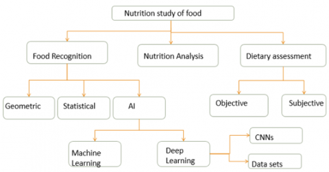
The system is broadly categorized into three major areas: food recognition from images, nutrient estimation, and various dietary assessment methods as shown in Figure 1. Food recognition is further divided into geometrical, statistical, and Artificial Intelligence (AI) methods, with AI methods encompassing both Machine Learning and Deep Learning approaches, specifically different CNN architectures. Additionally, the system elaborates on various food-related datasets and the methodologies employed for nutrient evaluation.
Figure 1. Different areas of nutrition study of food
2.1 Food recognition
Different methods are available to recognize the food images [3]. Feature-based methods were used previously for food image recognition. In previous studies, a variety of features have been utilized for image analysis, each serving distinct purposes. These attributes encompass a diverse set of features, including descriptors related to color such as SCD (Scalable Color Descriptor) and DCD (Dominant Color Descriptor) [4]. Texture descriptors, such as FDE (Fractal Dimension Estimation) and EBD (Entropy-Based Categorization) [5], along with features like Gabor-Based Image Decomposition (GBID) are also considered. Furthermore, the inclusion of local region features involves techniques like scale-invariant feature transforms and multi-scale dense SIFT [6]. These features collectively contribute to a comprehensive approach to image processing and recognition tasks. Geometric feature-based methods are implemented in different ways. Lowe [7] proposed an approach to converting the image to scale-invariant coordinates. A method of shape matching is suggested by Belongie et al. [8] identified a direct one-to-one correspondence between images in the dataset at the pixel level and the input image. Felzenszwalb [9] proposed a method using the concept of triangulation of polygons by decomposing objects into meaningful pieces. The limitation of the above methods is recognizing the features; for example, edges, contours, and key points are problematic. Statistical Feature methods for identifying food images are based on the spatial arrangement of ingredients on the food items. Yang et al. [10] introduced an innovative approach to food recognition. This method involves computing pairwise measurements among local features and executing image segmentation into eight distinct categories. Mapping each and every pixel with the ingredients is done for food identification. Hoashi et al. [11] introduced the idea of combining different image attributes, such as gradient histograms, Bag of Features, color, and Gabor features, using multiple kernel learning (MKL). Furthermore, Bosch et al. [12] have developed a strategy that integrates both global and local features to facilitate food identification.
The limitations of statistical methods are:
1) Cluttered images are not easy to handle.
2) Rigid systems are required when more categories of food images are used.
3) A greater number of food item groupings with lower accuracy.
For detecting food photos, machine learning and deep learning algorithms are frequently utilized. Algorithms are trained to autonomously identify connections and patterns within data and utilize this information for forecasting or decision-making. This procedure is often known as "Machine Learning (ML)," which is a branch of AI. By learning from examples and feedback, machine learning aims to develop algorithms that can gradually improve their performance on a task. The classification of objects is the main application of machine learning. Support Vector Machines are a traditional technique used for classification jobs like identifying foods. Images were classified using an SVM in a study by Zhang et al. [13]. An ensemble learning technique for classifying images is Random Forest. According to criteria such as color, texture, and shape, food photographs were classified using a random forest in a study by Sari et al. [14]. The term "multiple instance learning" (MIL) refers to a machine learning technique that can handle data that has many instances, such as food images that contain several food items. An MIL method was used to identify food items in photos in the publication " Describing objects by their attributes" by Farhadi et al. [15].
A sector within the realm of machine learning, referred to as deep learning (DL), involves training neural networks with several layers to discover data representations. DL models automatically learn characteristics from raw input data, such as text, audio, and images, by iteratively improving their predictions through a process known as backpropagation. As a result, deep learning models might be able to interpret natural language, recognize images, and recognize speech at the highest level possible. An instance of a deep learning model is CNN, designed specifically to excel in image recognition tasks.
A CNN architecture, as shown in Figure 2, comprises two primary components. The initial phase, known as feature extraction, involves the application of convolutional operations to identify and isolate distinctive attributes within an image for subsequent analysis. This process involves multiple sets of convolutional layers and pooling layers integrated into a network termed a feature extraction network. In the second phase, a fully-connected layer is made use of to harness the extracted features and the results of the convolutional process for the purpose of classifying the image. The underlying objective of this CNN feature extraction model is to distill the dataset into a minimal set of pertinent features. It accomplishes this by creating novel features through the amalgamation of original feature sets into a singular new attribute. As depicted in the architectural layout of the CNN, multiple levels of convolutional layers contribute to its structure [16].
Figure 2. Typical CNN architecture
Subhi and Ali [17] introduced an intricate convolutional model encompassing 24 layers. This architecture comprises a total of 21 convolutional layers in addition to 3 fully connected layers. They created a dataset with 11 categories of Malaysian food items and around 5400 images. Kagaya et al. [18] presented a CNN model named CNN-NIN for recognizing food by using images from three different methods, such as a) images from social media, b) images sourced from the FOOD 101 dataset, and c) images from the Caltech-256 dataset. The accuracy for the methods is 96%, 95%, and 99%, respectively. Lu [19] suggested a system using CNN on ten-class small-scale food image data and obtained an accuracy of 74%. Liu et al. [20] have introduced a valuable deep learning-powered food recognition system that leverages edge computing service infrastructure. For the FOOD 101 dataset, this system attained 94% accuracy, and the UEC100 dataset shows 95.2% accuracy [20]. Pandy et al. [21] proposed a system using a multifaceted CNN called Ensemble Net with an accuracy of 97.6% on the FOOD101 dataset.
Using transfer learning, Chaitanya et al. [22] offer a method for classifying food images using a CNN architecture with a pre-trained Inception v3 model. The model demonstrates effectiveness in identifying and classifying food photos, showcasing a 97.00% accuracy rate across 20 different food categories. Enhancements to the model's functionality and efficacy in providing nutritional information and promoting the adoption of healthy eating habits result from the utilization of data augmentation techniques and web crawlers for information extraction. The method's drawbacks, however, might include the need for a sizable and varied dataset to guarantee reliable training, the computational resources needed to train deep neural networks, and the difficulty of optimizing hyperparameters for best results across a wider variety of food classes. A faster R-CNN for identification of food using image recognition techniques is proposed by Nadeem et al. [23]. By combining region proposal networks (RPN) and a fast R-CNN-like network into one effective model, faster R-CNN does away with the requirement for outside proposal methods. Its open-source implementation, versatility, and end-to-end training make it a popular and efficient option for item detection in a range of applications. The technique just makes use of a dataset that has 16,000 food photos divided into 14 different kinds. Freitas et al. [24] conducted a study aimed at developing a system tailored for food recognition, achieved through the segmentation and image classification. With the use of image segmentation algorithms and deep learning techniques, the suggested system demonstrated efficacy in recognizing just nine food groups. The creation of a Brazilian food dataset was a significant addition to the study, and trials were carried out utilizing cutting-edge segmentation techniques to improve food segmentation accuracy.
The accuracy of food image recognition using various methods described in the related work is shown using a graphical representation in Figure 3.
Figure 3. Accuracy of food recognition
There are various obstacles to overcome when applying deep learning techniques, especially convolutional neural networks (CNNs), to food recognition tasks. These include the fact that deep learning is resource-intensive and requires a substantial amount of computational power for training; the challenge of optimizing hyperparameters across a variety of food classes; the dependence on large and diverse datasets for reliable performance and generalization; the impediments to identifying obscured or partially visible food items; the decreased applicability of deep learning in real-world scenarios because of background clutter and fluctuating lighting conditions; the high expense of annotating large-scale datasets for training. Resolving these issues will be crucial to improving deep learning-based food recognition systems' scalability, efficacy, and accuracy in real-world settings. All of these issues are addressed by the suggested system.
2.2 Dataset
The UECFOOD-100 dataset includes 100 distinct food categories, each of which has a bounding box that indicates the food item's positioning inside the image. Notably, a significant portion of the food categories within this dataset corresponds to prevalent Japanese culinary offerings [25]. A similar variation of UECFOOD-100 is UECFOOD-256. However, it differs in that it has 256 different food photos, which makes up more of the total amount of images. The 101,000 real-world photographs in Food-101 are divided into 101 different food categories. It includes a variety of dietary groups that look alike on the surface [26]. Similar to this, the 1098 food photos in the PFID food dataset come from 61 distinct categories. There are now three examples of 101 fast foods in the PFID collection [27]. UNCIT-FD1200 has 4754 pictures of food. The Food 5K dataset encompasses two distinct categories: "food" and "non-food," each containing a set of 500 images. The 4000 Indian cuisine images in the collection are divided into 80 different classes or categories. The Food-11 dataset encompasses 4,000 images of Indian food, categorized into 80 distinct classes or categories [28]. The Food-101 is a dataset with 101,000 total pictures and 101 different food categories. The dataset is made to be used for training and assessing computer vision models for food recognition tasks, and each image in it belongs to one of the food categories.
Nutrition analysis from food images using deep learning involves using CNNs to automatically identify and quantify the nutritional content of food in images. This approach can be used to help individuals track their dietary intake, as well as to aid researchers and healthcare professionals in assessing dietary patterns and evaluating interventions. A CNN model is trained on a sizable dataset of labeled food photos in this method, where the labels include both the food item and its associated nutritional information (e.g., calories, macronutrient composition). After the CNN has undergone training, it becomes capable of predicting the nutritional composition of novel food images. A pivotal obstacle in this endeavour involves precisely recognizing the food item depicted within the image, as this aspect significantly influences the precision of the predicted nutrient values. To address this challenge, researchers often use object detection or segmentation techniques in combination with CNNs, in order to first identify and isolate the food item before predicting its nutritional content. Overall, the use of DL for nutrition analysis from food images has the potential to revolutionize dietary assessment and monitoring, enabling more accurate and efficient evaluation of dietary patterns and interventions. The overall system architecture is shown in Figure 4.
Figure 4. Proposed architecture diagram
The following are the steps in the suggested system:
(1) The server receives the captured food image for preprocessing and recognition.
(2) The image is given to a pre-trained neural network.
(3) After CNN identifies the image, the server receives the label.
(4) Through the use of web crawling and Google searches, the food item's nutrients are estimated.
(5) An algorithm is proposed to calculate the Calorie information and compared the results with existing systems.
3.1 Experimental setup
The system is implemented using the NVIDIA GPU. This is the version of the NVIDIA driver that is installed on the system: a Tesla T4 with a driver version of 525.85.12 and a CUDA version of 12.0. NVIDIA GPUs may be used for general-purpose computing thanks to the parallel computing platform and programming model known as CUDA. The temperature of the GPU was 42°C. The current performance level of the GPU is P0. The power usage of the GPU and its power limit were 25W and 70W. The PCI bus ID of the GPU was 00000000:00:04.0.
3.2 Dataset: FOOD101
Lukas Bossard and colleagues generated the Food-101 dataset. The initial release took place in 2014. The dataset has been widely used in research on food recognition using computer vision [29]. This extensive dataset encompasses 101,000 images, each precisely categorized into one of the 101 diverse food classes. Each class, encapsulating a distinct food type, ranges from staple dishes to specific fruits, vegetables, desserts, and various international cuisines.
Noteworthy for its challenge in fine-grained recognition, the dataset prompts models to discern between visually similar or subtly different food items. The data collection process involves web scraping techniques, where images are sourced from the internet, fostering a realistic representation of food items encountered in everyday scenarios. The inclusivity of images, irrespective of professional quality or appearance, adds authenticity to the dataset.
One of the significant aspects of the Food-101 dataset is its openly accessible nature for research purposes. As an open resource, it has become a benchmark for training and evaluating deep learning models designed for food recognition. The dataset's availability has facilitated its widespread use in the development and assessment of algorithms, serving as a reference in numerous research papers within the domains of computer vision and deep learning.
Figure 5. Proposed architecture diagram
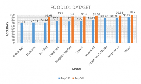
However, the dataset is not without its challenges. Potential class imbalances may exist, necessitating consideration during model training. Furthermore, the dataset's inherent variability, encompassing diverse settings, lighting conditions, backgrounds, and camera angles, poses challenges that models must overcome for robust performance. Figure 5 displays sample images from the Food-101 dataset as an illustration. Figure 6 depicts the accuracy using different deep learning models.
Figure 6. Accuracy of Food-101 dataset using different state-of art models
3.3 Preprocessing
A raw image comprises some elements that make it unsuitable for classification and identification, such as noise, environmental influences, insufficient resolution, and an undesirable backdrop. Enhancing the image quality and getting it ready for additional processing are crucial for accurate item identification. In this study, noise reduction and contrast enhancement make up the pre-processing step. A collection of techniques commonly known as "data augmentation" can be harnessed to artificially augment the volume of data by creating extra data instances from the existing dataset. This process entails utilizing deep learning models to introduce new data instances or applying minor alterations to the existing data. Some of the activities for data augmentation [30, 31] are described below:
3.3.1 Shear transformation
It is a technique for 2-D affine transformation. The sheer change slants the contour of the picture. Shear transformation diverges from rotation by keeping one axis constant while distorting the image at a specific angle known as the shear angle. This introduces a concealed "stretch" effect to the image that isn't apparent in rotations. The parameter shear_range designates the degree of slant angle.
The transformation matrix for the shear transform is given below:
$\begin{array}{lll}{[1} & \text { shearx } & 0 \\ {[\text { sheary }} & 1 & 0] \\ {[0} & 0 & 1]\end{array}$ (1)
We have "shearx" in this context, to apply the shear factor along the x-axis, and to apply the shear factor along the y-axis, we have "sheary".
To apply the shear transformation to a 2D point P=(x1, y1), we can represent the point as a 3x1 column vector [x1, y1, 1] and multiply it by the shear transformation matrix to obtain the transformed point P'=(x1', y1'):
$\begin{aligned}
& {\left[\mathrm{x}_1^{\prime}\right] \quad\left[\begin{array}{lll}
1 & \mathrm{a} & 0
\end{array}\right] \quad\left[\mathrm{x}_1\right]} \\
& {\left[\mathrm{y}_1^{\prime}\right]=\left[\begin{array}{lll}
\mathrm{b} & 1 & 0
\end{array}\right] *\left[\begin{array}{l}
\mathrm{y}_1
\end{array}\right]} \\
& {[1] \quad\left[\begin{array}{lll}
0 & 0 & 1
\end{array}\right] \quad[1]}
\end{aligned}$ (2)
The resulting transformed point P' has coordinates x1' and y1' given by:
$\begin{aligned} & {\mathrm{x}}_1^{\prime}=\mathrm{x}_1+\mathrm{a}^* \mathrm{y}_1 \\ & \mathrm{y}_1^{\prime}=\mathrm{y}_1+\mathrm{b}^* \mathrm{x}_1\end{aligned}$ (3)
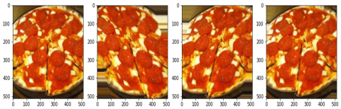
This transformation shears the original point ‘P’ in the ‘x1’ direction by an amount proportional to its ‘y’ coordinate, and in the ‘y1’ direction by an amount proportional to its ‘x’ coordinate. Sample image from food101 dataset with shear range=30 is represented in Figure 7.
Figure 7. Sample image with shear range=30
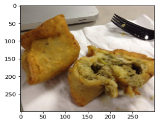
Figure 8. Sample image after horizontal and vertical flip
3.3.2 Flipping
The pixels will be reversed row- or column-wise, depending on the direction of the vertical and horizontal flip augmentation. The mathematical equation for horizontal flipping is:
$\begin{aligned}
& {\left[\mathrm{x}_1{ }^{\prime}\right] \quad\left[\begin{array}{lll}
-1 & 0 & \mathrm{w}-1]
\end{array}\left[\mathrm{x}_1\right]\right.} \\
& {\left[\mathrm{y}_1{ }^{\prime}\right]=\left[\begin{array}{lll}
0 & 1 & 0
\end{array}\right]^*\left[\mathrm{y}_1\right]} \\
& {[1]\left[\begin{array}{lll}
0 & 0 & 1
\end{array}\right] \quad[1]}
\end{aligned}$ (4)
where, the image width is represented by “w”. The image is horizontally flipped as a result of this transformation, making the right side the left side and vice versa. The x coordinate of each pixel is negated and then translated by w-1 to the opposite side of the image. The y coordinate of each pixel is unchanged. The mathematical equation for vertical flipping is:
$\begin{aligned}
& \left.\left[\mathrm{x}_1^{\prime}\right] \quad \begin{array}{lll}
{[1} & 0 & 0
\end{array}\right] \quad\left[\mathrm{x}_1\right] \\
& {\left[\mathrm{y}_1^{\prime}\right]=\left[\begin{array}{lll}
0 & -1 & \mathrm{~h}-1
\end{array}\right] *\left[\begin{array}{ll}
\mathrm{y}_1
\end{array}\right]} \\
& {[1] \quad\left[\begin{array}{lll}
0 & 0 & 1]
\end{array}[1]\right.}
\end{aligned}$ (5)
where, h is the image's height. With this transformation, the bottom of the image becomes the top and vice versa. The x coordinate of each pixel is unchanged. The y coordinate of each pixel is negated and then translated by h-1 to the opposite side of the image. Sample image and output after applying horizontal and vertical flip is depicted in Figure 8.
3.3.3 Scaling
The mathematical function for scaling an image by a scaling factor s can be written as:
If the original image has dimensions (x1, y1), then the scaled image will have dimensions (s*x1, s*y1). In practice, the scaling factor s is often chosen randomly within a certain range during data augmentation. For example, if we want to randomly scale an image by a factor between 0.8 and 1.2, we can choose a number r which is in between 0.8 and 1.2 randomly and set s=r. Then, the above equation can be used to compute the dimensions of the scaled image as (s*x1, s*y1). Finally, apply an interpolation algorithm, such as bilinear or nearest neighbor interpolation, to resize the original image to the computed dimensions and obtain the scaled image.
Many deep learning frameworks provide built-in functions for scaling images during data augmentation, which take care of the above steps automatically. Setting min_scale=.75 means that the smallest dimension of the input images will be resized to 75% of their original size. For example, if an input image has dimensions (100, 200), the smallest dimension is 100, so it will be resized to 75% of its original size, which is 75. The resulting image dimensions will be (75, 150). This can be useful for preventing input images from being too small, which can result in a loss of detail and accuracy in the trained model. By setting a minimum scale, we can ensure that all input images are at least a certain size while still preserving their aspect ratios.
3.4 NutriFoodNet
Following the acquisition of the image datasets, various data augmentation techniques were used as preprocessing. We developed a framework for deep CNN to recognize and detect images of food. The recognition model takes the image of a food image as input and finds a label as a text class that describes the food item as the output. The neural network assigns a single class label to the input image. The architecture created for this research study is called NutriFoodNet. Together with this study, a comparison of the following CNN designs is also conducted.
Resnet-18: A convolutional neural network architecture with 18 layers, is composed of one input layer, four convolutional layers, four pooling layers, and one fully connected layer. The input layer has dimensions of 224 × 224 × 3, where 3 represents the number of RGB channels. The pooling layers utilize a max pooling function with a pool size of 2 × 2, and the convolutional layers employ a 3 × 3 kernel size. The fully connected layer employs the softmax activation function, producing a probability distribution across the output classes. To address the challenge of vanishing gradients in deep neural networks, ResNet-18 incorporates identity mappings or skip connections [32].
Resnet-50: ResNet-50 is the name of a deep convolutional neural network with 50 layers. It has 1,000 item categories for categorizing photos. The network's input measures 224 by 224 by 3. The network is divided into multiple phases, each of which includes a number of residual blocks. In the first step, a convolutional layer comes before a max-pooling layer. In the second stage, there are 3 residual blocks. Each block consists of 2 convolutional layers. The third stage of the network comprises four residual blocks, the fourth stage includes six, and the fifth stage incorporates three. The upper layers of the network consist of a fully connected layer, a softmax layer, and a global average pooling layer.
Inception v3: Google created the convolutional neural network architecture known as Inception v3. It is intended to identify images by extracting information across numerous convolutional layers and comprises 48 layers. The network has a number of specialized convolutional layers, including Inception modules that concatenate the outputs of several convolutions and 1×1 convolutional layers that serve as bottleneck layers. The ImageNet dataset, which has millions of annotated images, was used to train Inception v3, which at the time of its release produced state-of-the-art results. Although the architecture can be altered to accept images of other sizes, Inception v3 requires input images to be 299 by 299 pixels in size [33].
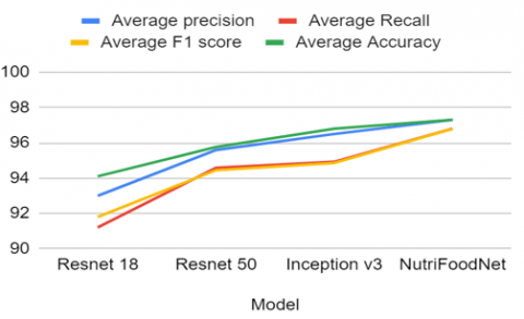
To evaluate the performance of the food recognition system, the above mentioned models were employed. Among these, the Inception V3 Model emerged as the most effective, leading to the adoption of a modified architecture in NutriFoodNet, incorporating additional augmentation methods for preprocessing. The learning rates of the models were compared with those of NutriFoodNet. The average accuracy, precision, recall, and F1 score of all models were computed and juxtaposed with the performance of the proposed model.
T-tests are used to compare the performance of different CNN models. The performance metric to evaluate the CNN model is decided as accuracy. Based on the results of the T-test, it is possible to determine whether there is a statistically significant difference in performance between the CNN models. If the p-value of the T-test is below a chosen significance level (e.g., 0.05), the null hypothesis can be rejected and conclude that there is a significant difference in performance. the p-value obtained for the comparisons is less than 0.05 and is shown in Table 1 below:
Table 1. Result of T-test
|
Comparison |
NutriFood Net- ResNet18 |
NutriFood Net- ResNet50 |
NutriFood Net- InceptionV3 |
|
T-statistic |
30.94663553 |
11.29343159 |
3.958898771 |
|
P-value |
3.43E-78 |
3.38E-23 |
1.05E-04 |
3.4.1 Architecture overview and layer configuration of NutriFoodNet
The Inception 3 architecture is modified to create NutriFoodNet, our convolutional neural network architecture. The first distinction is that noise was reduced during processing so that the original images, which had a length of 512 pixels for one side, were scaled to 299 pixels before the first layer. The second distinction is that NutriFoodiNet starts its neural network with an extra convolutional layer to learn more about the features in the pictures. Configurations of layers in the proposed model are shown in Table 2.
Table 2. Layer configurations
|
Layer Type |
Output Shape |
|
Input Conv2D BatchNormalization Activation Conv2D BatchNormalization Activation MaxPooling2D GlobalAveragePooling2D Dense layer Dropout Dense layer |
(None, 299, 299, 3) (None, None, None, 32) (None, None, None, 32) (None, None, None, 32) (None, None, None, 32) (None, None, None, 32) (None, None, None, 32) (None, None, None, 32) (None, 2048) (None, 128) (None, 128) (None, 101) |
|
Total parameters 22,065,314 Trainable parameters 22,030,882 Non-trainable parameters 34,432 |
|
3.4.2 Optimization techniques
NutriFoodNet uses standard optimization techniques, such as Adam Optimizer, for training. To speed up training, techniques like batch normalization are employed to normalize the inputs to each layer during training. The optimization algorithm used in Inception v3, and in many deep learning models, is typically a variant of stochastic gradient descent (SGD). One common variant is the Adam optimizer. The mathematical equations for the Adam optimizer are as follows:
The Adam update rule for each parameter θi at time step t is given by:
$m t=\beta 1 \cdot m t-1+(1-\beta 1) \cdot g t$ (6)
$v t=\beta 2 \cdot v t-1+(1-\beta 2) \cdot g t 2$ (7)
Bias-corrected moment estimates:
$\widehat{m t}=\frac{m t}{1-\beta 1^t}$ (8)
$\widehat{v t}=\frac{v t}{1-\beta 2^t}$ (9)
Update rule:
$\theta_t=\theta_{t-1}-\alpha \cdot \frac{\widehat{m t}}{\sqrt{v t}+\epsilon}$ (10)
where, Model parameters defined by θ, for the parameters at the time step, gradient of the objective function represented by gt, learning rate by α, exponential decay rates for the moment estimates sare β1 and β2. First moment estimate, that is, the mean of the gradients is represented by mt. Second moment estimate that is, uncentered variance of the gradients, is vt, and ϵ represents a small constant to prevent division by zero. These equations define how the parameters of the model are updated during training using the Adam optimizer. The algorithm adapts the learning rates for each parameter based on their historical gradients, helping to achieve faster convergence and better generalization.
3.4.3 Activation function
The Rectified Linear Unit (ReLU) serves as a commonly utilized activation function in neural networks, especially for hidden layers. Its pivotal function lies in introducing non-linearity to the model, allowing the network to capture complex patterns and relationships. ReLU is expressed using the mathematical expression as follows:
$f(x)=\max (0, x)$ (11)
In this equation, the input to the function is denoted by ‘x’, and ‘max’ denotes the element-wise maximum operator.
The ReLU activation function returns x if it is positive; otherwise, it outputs zero. Visually, it resembles a ramp, permitting positive values to remain unaltered while setting negative values to zero. ReLU's simplicity and non-linearity enhance computational efficiency and help address the vanishing gradient problem, setting it apart from activation functions such as sigmoid or tanh.
3.4.4 Loss function
The concluding classification layer of NutriFoodNet employs the softmax cross-entropy loss function. The mathematical representation for the loss function is detailed as follows:
The softmax cross-entropy loss for a single example is calculated as:
$\begin{aligned} & \text { Softmax Cross - Entropy Loss } -\sum_i y_i \log \left(\widehat{y}_i\right)\end{aligned}$ (12)
where, yi is the true label (ground truth) for class i (if the sample belongs to class i then 1, otherwise 0) and $\widehat{y}_t$ is the predicted probability of the sample belonging to class i from the softmax activation. In this Eq. (12), the sum is taken over all classes. The loss is penalized more heavily when the predicted probability diverges from the true label. The goal during training is to minimize this loss across all examples in the training set. For a batch of examples, the average softmax cross-entropy loss is often used.
$\begin{aligned} & \text { Average Softmax Cross-Entropy Loss } =\frac{1}{N} \sum_j \sum_i y_{i j} \log \left(y_{i j}\right)\end{aligned}$ (13)
where, N is the batch size and j indexes the examples in the batch. This loss function encourages the model to assign high probabilities to the correct classes. The logarithmic term penalizes the model more if the predicted probability is far from the true label, contributing to effective learning during training.
3.5 Hyperparameter fine-tuning
The transfer learning model has the advantages of learning more quickly than models created from scratch and allowing the last layers of the model to be trained for more accurate categorization. For several pre-trained models, initial standardizations of the hyperparameters were carried out. Table 3 is a list of the specifics of the hyperparameter setting.
In the CNN architecture, the learning rate hyperparameter plays a crucial role in regulating the step size during each optimization iteration. This rate, determined by the estimated error gradient, governs the scale of the update applied to the model weights. Typically chosen as a moderate value like 0.1, 0.01, or 0.001, it may be adjusted based on the model's performance on a validation set. The learning rates for various architectures are depicted in Figure 9.
Table 3. Hyperparameter specifications
|
Hyper Parameters |
|
|
Dropout Epochs Activation Function Regularization Optimizer Learning rate Output classes |
0.3 50 ReLu Batch Normalization Adam 0.001 101 |
Figure 9. Learning rate of CNN architectures
Figure 10. RGB channels of sample image
The input shape of the model is 32 × 3 × 299 × 299, which means that we are feeding 32 images with 3 channels (RGB) and size 299 × 299 pixels each. RGB channel of a sample image is shown in Figure 10.
Here we create an ImageDataLoaders object for the image classification task from a folder of images located at path. Sets for training and validation are separated from the dataset. using 20% of the images as a validation set (valid_pct=0.2). The data is augmented during training using a set of random transformations provided in batch_tfms. Specifically, the images are resized to 299 × 299 (Resize(299)), and a set of augmentations such as flipping, rotation, and zooming are applied. Finally, the images are normalized using the statistics of the ImageNet dataset (Normalize.from_stats(*imagenet_stats)). A batch size of 32 is used (bs=32).
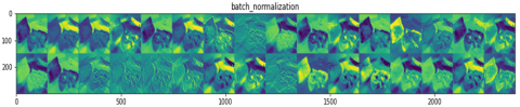
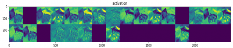
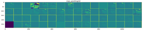
The output of each layer, such as convolution, batch normalization, activation, and max pooling, for the sample image is shown in Figure 11 below:
(a) RGB sample image
(b) con2D
(c) batch normalization
(d) activation
(e) max_pooling
Figure 11. Output of different layers
3.6 Performance analysis
3.6.1 Accuracy
The accuracy of the CNN model is computed mathematically as:
Accuracy $=\frac{(T p+T n)}{(T p+T n+F p+F n)}$ (14)
where, Tp: True positive; Tn: True negative; Fp: False Positive; Fn: False Negative.
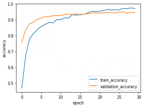
The train and validation accuracy, train and validation loss for the proposed architecture, NutrifoodNet, are shown in Figure 12.
(a) Train and validation accuracy
(b) Train and validation loss
Figure 12. Accuracy and loss of NutriFoodNet
3.6.2 Confusion matrix
To evaluate a classifier's performance, a confusion matrix is employed. Below is a breakdown of how many of the model's predictions are Tp, Tn, Fp, and Fn. Confusion matrix for sample 13 classes is shown in Figure 13.
Figure 13. Confusion matrix
3.6.3 Precision
The precision of the classifier is articulated mathematically as:
Precision $=\frac{T p}{(T p+F p)}$ (15)
3.6.4 Recall
Recall, alternatively referred to as sensitivity or the true positive rate, is calculated by dividing the number of true positive predictions (instances correctly identified as the positive class) by the total count of actual positive instances (comprising true positives and false negatives). Mathematically, this is articulated as:
Recall $=\frac{T p}{(T p+F n)}$ (16)
3.6.5 F1 score
The F1 score evaluates a classifier's performance and the mathematical representation for computation is expressed as:
$F 1$ Score $=\frac{2 *(\text { Precision } * \text { Recall })}{(\text { Precision }+ \text { Recall })}$ (17)
The proposed NutriFoodNet model undergoes evaluation, comparison, and visualization of its average precision, recall, F1 score, and accuracy, as depicted in Figure 14.
Figure 14. Performance analysis of NutriFoodNet
The USDA National Nutrient Database, an online nutrient database, can be used to search up the nutritional details for an item from the item-101 dataset. Here is a step-by-step procedure for carrying this out.
(1) Enter the name of the food recognized by using the proposed architecture to search the USDA National Nutrient Database. Sending a query to the database's API will enable you to accomplish this, and the API will respond with a list of foods that fit the query.
(2) Using the food's description and/or additional details, choose the appropriate item from the list.
(3) Obtain from the database the nutritional data for the chosen food. The nutritional information often contains details about serving size, calories, macronutrients, micronutrients, and other nutrients and is presented in a standardized manner, such as a table.
(4) Extract the pertinent nutritional data from the nutrient table and present it in a way that is easy for users to understand, such as a table or a chart.
The nutrient content of sample food items from the Food 101 dataset is shown in Table 4 below:
Table 4. Nutrient contents of sample food items
|
Sl. No |
Name |
Protein |
Calcium |
Fat |
Carbohydrates |
|
0 |
apple pie |
2.63 |
0.018 |
14.04 |
35.09 |
|
1 |
baby back ribs |
18.75 |
0.026 |
9.82 |
0 |
|
2 |
baklava |
6.64 |
0.04 |
29.13 |
37.53 |
|
3 |
beef carpaccio |
27.1 |
0.012 |
14.93 |
0 |
|
4 |
beef tartare |
15.67 |
0.032 |
13.84 |
1.56 |
|
5 |
beet salad |
1.32 |
0.018 |
5.29 |
11.01 |
The proposed algorithm is designed to calculate the calories for multiple food items based on their nutritional information. The core of the algorithm is encapsulated in the calculateCaloriesForMultipleItems function. This function takes a list of food items from the food101 dataset, where each item is represented by a dictionary containing information about carbohydrates, proteins, and fats. For each food item, the algorithm checks to see if complete nutritional information is available. If so, it extracts the values for carbohydrates, proteins, and fats and calculates the calories using the formula: calories = (carbohydrates * 4) + (proteins * 4) + (fats * 9). The calculated calories are then appended to a results list. In cases of missing or incomplete nutritional information, an error message is appended to the results. The function ultimately returns a list of calculated calories or error messages for each food item.
Beyond the function, the algorithm demonstrates an example usage by reading data from an Excel file into a Pandas DataFrame. The DataFrame is then converted into a list of dictionaries, which is subsequently passed to the calculateCaloriesForMultipleItems function. The calculated results are stored in the calories results list, and the algorithm concludes by displaying the results for each food item. The pseudocode for the proposed algorithm is given below:
Algorithm calculateCaloriesForMultipleItems(foodItems):
results = []
// List to store the calculated calories for each food item
FOR EACH nutritionTable IN foodItems:
IF "Carbo" IN nutritionTable AND "Proteins"
IN nutritionTable AND "Fats"
IN nutritionTable:
carbohydrates = nutritionTable[“carbo”]
proteins = nutritionTable["Proteins"]
fats = nutritionTable["Fats"]
// Calories calculation
calories = (carbo * 4)+(proteins * 4) + (fats * 9)
results.append(calories)
ELSE:
// Handle missing information in the nutrition table
results.append("Error:Incomplete information")
RETURN results
// Read data from Excel file into a DataFrame
excel_file_path = 'path/to/your/excel/file.xlsx'
df = READ_EXCEL(excel_file_path)
// Convert DataFrame to a list of dictionaries
// Each dictionary represents a row in the Excel file
foodItemsList = CONVERT_TO_DICT(df, orient='records')
// Example usage with the data read from the Excel file
caloriesResults=calculateCaloriesForMultipleItems(foodIte
msList)
// Display results
FOR i FROM 0 TO LENGTH(caloriesResults) - 1:
PRINT("Food Item " + (i + 1) + ": " + caloriesResults[i] + "
calories")
Calculated calories for the above food items are compared with the existing database such as nutritionix and nutrition value. The graph given in Figure 15 shows the result.
Figure 15. Comparison of calorie calculation
The Mean Absolute Percentage Error (MAPE), and the RMSE, or Root Mean Square Error for each food item are employed as evaluation metrics for the proposed methodology [34].
MAPE $=\frac{1}{n} \sum_{i=1}^n \frac{C_{\text {pred }}-C_{\text {real }}}{C_{\text {real }}} * 100$ (18)
$R M S E=\frac{1}{n} \sqrt{\sum_{i=1}^n\left(C_{\text {pred }}-C_{\text {real }}\right)^2}$ (19)
where, n is the matching records for each food item included in the created dataset, Cpred is the predicted calorie of the food, and Creal is the actual calorie. Overall, the following evaluation metrics are used to estimate the caloric content of 101 distinct dishes from the Food101 image dataset:
$M A P E_{\text {overall }}=\frac{1}{101} \sum_{i=1}^{101} M A P E_i$ (20)
$R M S E_{\text {overall }}=\frac{1}{101} \sum_{i=1}^{101} R M S E_i$ (21)
Figure 16. Comparison of MAPE and RMSE
MAPE and RMSE for the proposed model is compared with the same using Nutritionix and Nutritionvalue and shown in Figure 16.
A streamlined architecture for food recognition employing convolutional neural networks (CNNs) has been introduced. The proposed architecture includes a pre-processing step that involves resizing the input images and applying image augmentation techniques to improve the model's robustness. The suggested architecture has been tested on the Food-101 dataset and outperformed numerous other cutting-edge techniques in terms of food recognition, achieving high accuracy. The outcomes demonstrate that the suggested CNN architecture can accurately recognize food items from images, which can help people make more informed decisions about their food choices. Future work in this area could focus on developing more user-friendly interfaces for the system to make it more accessible to the general public. Additionally, research could focus on developing personalized nutrition plans based on individual health needs and preferences. Overall, continued research and development in this area can help to promote healthy eating habits and improve the overall health and well-being of individuals around the globe.
[1] World Health Organization, Nutrition. (2022). WHO global Nutrition report. https://www.who.int/health-topics/nutrition.
[2] Liu, C., Cao, Y., Luo, Y., Chen, G., Vokkarane, V., Ma, Y. (2016). DeepFood: Deep learning-based food image recognition for computer-aided dietary assessment. In Inclusive Smart Cities and Digital Health: 14th International Conference on Smart Homes and Health Telematics, ICOST 2016, Wuhan, China, pp. 37-48. https://doi.org/10.1007/978-3-319-39601-9_4
[3] Sreetha, E.S., Naveen Sundar, G., Narmadha, D. (2022). Comparative study on recognition of food item from images for analyzing the nutritional contents. In Disruptive Technologies for Big Data and Cloud Applications: Proceedings of ICBDCC 2021, pp. 269-276. https://doi.org/10.1007/978-981-19-2177-3_27
[4] Wong, K.M., Po, L.M., Cheung, K.W. (2007). Dominant color structure descriptor for image retrieval. In 2007 IEEE International Conference on Image Processing, San Antonio, TX, USA, pp. VI-365. https://doi.org/10.1109/ICIP.2007.4379597
[5] Bosch, M., Zhu, F., Khanna, N., Boushey, C.J., Delp, E.J. (2011). Food texture descriptors based on fractal and local gradient information. In 2011 19th European Signal Processing Conference, pp. 764-768.
[6] He, Y., Xu, C., Khanna, N., Boushey, C.J., Delp, E.J. (2014). Analysis of food images: Features and classification. In 2014 IEEE International Conference on Image Processing (ICIP), Paris, France, pp. 2744-2748. https://doi.org/10.1109/ICIP.2014.7025555
[7] Lowe, D.G. (2004). Distinctive image features from scale-invariant keypoints. International Journal of Computer Vision, 60: 91-110. https://doi.org/10.1023/B:VISI.0000029664.99615.94
[8] Belongie, S., Malik, J., Puzicha, J. (2000). Shape context: A new descriptor for shape matching and object recognition. Advances in Neural Information Processing Systems, 831-837.
[9] Felzenszwalb, P.F. (2005). Representation and detection of deformable shapes. IEEE Transactions on Pattern Analysis and Machine Intelligence, 27(2): 208-220. https://doi.org/10.1109/TPAMI.2005.35
[10] Yang, S., Chen, M., Pomerleau, D., Sukthankar, R. (2010). Food recognition using statistics of pairwise local features. In 2010 IEEE Computer Society Conference on Computer Vision and Pattern Recognition, San Francisco, CA, USA, pp. 2249-2256. https://doi.org/10.1109/CVPR.2010.5539907
[11] Hoashi, H., Joutou, T., Yanai, K. (2010). Image recognition of 85 food categories by feature fusion. In 2010 IEEE International Symposium on Multimedia, Taichung, Taiwan, pp. 296-301. https://doi.org/10.1109/ISM.2010.51
[12] Bosch, M., Zhu, F., Khanna, N., Boushey, C.J., Delp, E.J. (2011). Combining global and local features for food identification in dietary assessment. In 2011 18th IEEE International Conference on Image Processing, Brussels, Belgium, pp. 1789-1792. https://doi.org/10.1109/ICIP.2011.6115809
[13] Zhang, C., Wang, T., Atkinson, P. M., Pan, X., Li, H. (2015). A novel multi-parameter support vector machine for image classification. International Journal of Remote Sensing, 36(7): 1890-1906. https://doi.org/10.1080/01431161.2015.1029096
[14] Sari, Y.A., Utaminingrum, F., Adinugroho, S., Dewi, R.K., Adikara, P.P., Wihandika, R.C., Mutrofin, S., Izzah, A. (2019). Indonesian traditional food image identification using random forest classifier based on color and texture features. In 2019 International Conference on Sustainable Information Engineering and Technology (SIET), Lombok, Indonesia. pp. 206-211. https://doi.org/10.1109/SIET48054.2019.8986058
[15] Farhadi, A., Endres, I., Hoiem, D., Forsyth, D. (2009). Describing objects by their attributes. In 2009 IEEE Conference on Computer Vision and Pattern Recognition, Miami, FL, USA, pp. 1778-1785. https://doi.org/10.1109/CVPR.2009.5206772
[16] Mishra, M. (2020). Towards data science, convolutional neural netorks explained. https://towardsdatascience.com/convolutional-neural-networks-explained-9cc5188c4939, accessed on August 27, 2020.
[17] Subhi, M.A., Ali, S.M. (2018). A deep convolutional neural network for food detection and recognition. In 2018 IEEE-EMBS Conference on Biomedical Engineering and Sciences (IECBES), Sarawak, Malaysia, pp. 284-287. https://doi.org/10.1109/IECBES.2018.8626720
[18] Kagaya, H., Aizawa, K., Ogawa, M. (2014). Food detection and recognition using convolutional neural network. In Proceedings of the 22nd ACM International Conference on Multimedia, pp. 1085-1088. https://doi.org/10.1145/2647868.2654970
[19] Lu, Y. (2016). Food image recognition by using convolutional neural networks (CNNs). arXiv preprint arXiv:1612.00983. https://doi.org/10.48550/arXiv.1612.00983
[20] Liu, C., Cao, Y., Luo, Y., Chen, G., Vokkarane, V., Ma, Y.S., Chen, S.P., Hou, P. (2017). A new deep learning-based food recognition system for dietary assessment on an edge computing service infrastructure. IEEE Transactions on Services Computing, 11(2): 249-261. https://doi.org/10.1109/TSC.2017.2662008
[21] Pandey, P., Deepthi, A., Mandal, B., Puhan, N.B. (2017). FoodNet: Recognizing foods using ensemble of deep networks. IEEE Signal Processing Letters, 24(12): 1758-1762. https://doi.org/10.1109/LSP.2017.2758862
[22] Chaitanya, A., Shetty, J., Chiplunkar, P. (2023). Food image classification and data extraction using convolutional neural network and web crawlers. Procedia Computer Science, 218: 143-152. https://doi.org/10.1016/j.procs.2022.12.410
[23] Nadeem, M., Shen, H., Choy, L., Barakat, J.M.H. (2023). Smart diet diary: Real-Time mobile application for food recognition. Applied System Innovation, 6(2): 53. https://doi.org/10.3390/asi6020053
[24] Freitas, C.N., Cordeiro, F.R., Macario, V. (2020). Myfood: A food segmentation and classification system to aid nutritional monitoring. In 2020 33rd SIBGRAPI Conference on Graphics, Patterns and Images (SIBGRAPI), Porto de Galinhas, Brazil, pp. 234-239. https://doi.org/10.1109/SIBGRAPI51738.2020.00039
[25] Matsuda, Y., Yanai, K. (2012). Multiple-food recognition considering co-occurrence employing manifold ranking. In Proceedings of the 21st International Conference on Pattern Recognition (ICPR2012), Tsukuba, Japan, pp. 2017-2020.
[26] Kawano, Y., Yanai, K. (2014). Foodcam-256: A large-scale real-time mobile food recognition system employing high-dimensional features and compression of classifier weights. In Proceedings of the 22nd ACM International Conference on Multimedia, pp. 761-762. https://doi.org/10.1145/2647868.2654869
[27] Chen, M., Dhingra, K., Wu, W., Yang, L., Sukthankar, R., Yang, J. (2009). PFID: Pittsburgh fast-food image dataset. In 2009 16th IEEE International Conference on Image Processing (ICIP), Cairo, Egypt, pp. 289-292. https://doi.org/10.1109/ICIP.2009.5413511
[28] Şengür, A., Akbulut, Y., Budak, Ü. (2019). Food image classification with deep features. In 2019 International Artificial Intelligence and Data Processing Symposium (IDAP), Malatya, Turkey, pp. 1-6. https://doi.org/10.1109/IDAP.2019.8875946
[29] Bossard, L., Guillaumin, M., Van Gool, L. (2014). Food-101–mining discriminative components with random forests. In Computer vision–ECCV 2014: 13th European conference, Zurich, Switzerland, pp. 446-461. https://doi.org/10.1007/978-3-319-10599-4_29
[30] Mumuni, A., Mumuni, F. (2022). Data augmentation: A comprehensive survey of modern approaches. Array, 16: 100258. https://doi.org/10.1016/j.array.2022.100258
[31] Mikołajczyk, A., Grochowski, M. (2018). Data augmentation for improving deep learning in image classification problem. In 2018 International Interdisciplinary PhD Workshop (IIPhDW), Świnouście, Poland, pp. 117-122. https://doi.org/10.1109/IIPHDW.2018.8388338
[32] He, K., Zhang, X., Ren, S., Sun, J. (2016). Deep residual learning for image recognition. In 2016 IEEE Conference on Computer Vision and Pattern Recognition (CVPR), Las Vegas, NV, USA, pp. 770-778. https://doi.org/10.1109/CVPR.2016.90
[33] Szegedy, C., Vanhoucke, V., Ioffe, S., Shlens, J., Wojna, Z. (2016). Rethinking the inception architecture for computer vision. In 2016 IEEE Conference on Computer Vision and Pattern Recognition (CVPR), Las Vegas, NV, USA, pp. 2818-2826. https://doi.org/10.1109/CVPR.2016.308
[34] Konstantakopoulos, F.S., Georga, E.I., Fotiadis, D.I. (2023). A novel approach to estimate the weight of food items based on features extracted from an image using boosting algorithms. Scientific Reports, 13(1): 21040. https://doi.org/10.1038/s41598-023-47885-0