Multiple-Image Encryption Using Sine Quadratic Polynomial Mapping and U-Shaped Scanning Techniques

SQPM represents an innovative one-dimensional chaotic map, ingeniously amalgamating the traditional sine map with a quadratic polynomial. The mathematical representation of SQPM is given in Eq. (1):

$x_{n+1}=\sin \left(\pi\left(e^{a+10}+b\right)\left(x_n^2+x_n+c\right)\right)$           (1)

where, $x_n \in(-1,1)$ denotes the initial value, $a, b, c \in[0, \infty)$ signify the control parameters, and $e$ is Euler's number. As a classical member of the 1D chaotic maps family, the sine map is known for its ability to generate chaotic sequences efficiently, albeit with a low computational cost. However, its major limitation lies in having a single control parameter with an exceedingly narrow chaotic range. The introduction of SQPM marks a significant advancement by expanding the number of control parameters available for image encryption algorithms to three. This enhancement allows SQPM to produce chaotic sequences of substantial complexity while maintaining minimal computational power $\forall a, b, c \in[0, \infty)$.

2.1 2D and 3D phase diagrams

The 2D and 3D phase diagrams for the sine map and SQPM are depicted in Figure 1. Figures 1a) and 1d) clearly show that the sine map exhibits a parabolic trajectory, occupying only a limited region of the 2D plane and 3D space. In contrast, SQPM does not adhere to a specific trajectory. Instead, it extensively covers a significant portion of both the 2D plane and 3D space when iterated with varying control parameters, such as a=b=c=0 or a=5, b=3, c=15. This expansive coverage by SQPM illustrates its superior capability in generating random sequences with greater randomness compared to the sine map.

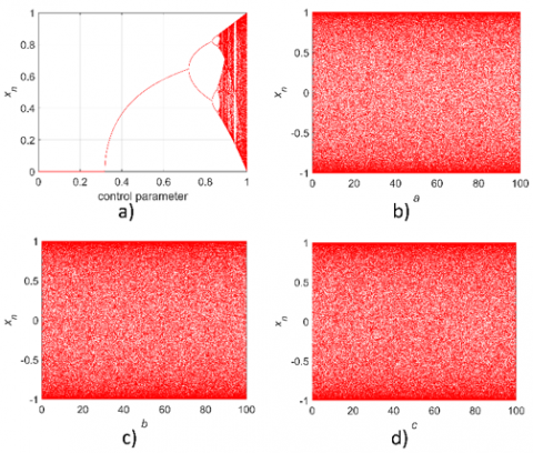
2.2 Bifurcation diagrams

A bifurcation diagram is a powerful tool for visualizing the evolution of a chaotic map's dynamic behavior as its control parameters change. Figure 2 showcases the bifurcation diagrams of both the sine map and SQPM. The sine map transitions into a chaotic regime when its control parameter lies within the range of [0.87, 1]. Notably, even within this chaotic regime, periodic windows are evident, as demonstrated in Figure 2a). The sine map only generates chaotic values across the range of (0,1) when its control parameter equals one. In stark contrast, SQPM exhibits a broader range of dynamic behaviors. As seen in Figures 2b), 2c), and 2d), SQPM consistently maps its input within the range of [-1,1] across all its control parameter values. Unlike the sine map, which is confined to a limited range of control parameters for chaotic behavior, SQPM demonstrates chaotic dynamics $\forall a, b, c \in[0, \infty)$ over an expanded parameter range. In essence, the inherent chaotic behavior of the sine map is substantially enhanced through the implementation of SQPM.

Figure 1. Phase diagrams: a), d) sine map (control parameter is 1); b), e) SQPM (a=b=c=0); c), f) SQPM (a=5, b=3, c=15)

2.png

Figure 2. Bifurcation diagrams: a) sine map, b) SQPM $(a \in[0,100], b=c=0), \mathrm{c}) \operatorname{SQPM}(b \in[0,100], a=c=0), d) \operatorname{SQPM}(c \in[0,100], a=b=0)$

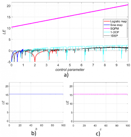
2.3 Lyapunov exponent

The Lyapunov exponent (LE) serves as a crucial measure for quantifying the rate at which two neighboring trajectories, originating from extremely close initial conditions, diverge. A positive LE value signifies chaotic behavior and a high sensitivity to initial conditions. Figure 3a) illustrates the LE values of SQPM in comparison with other chaotic maps such as the logistic map, the sine map, the one-dimensional cosine polynomial map (1-DCP) [40], and the one-dimensional sine-powered chaotic map (1-DSP) [41], plotted against a control parameter. Given that a higher LE value is indicative of superior chaotic performance [42], the LE calculations of SQPM clearly demonstrate its exceptional performance over traditional and other recently developed chaotic maps. Distinctively, SQPM consistently exhibits positive LE values, indicating an absence of non-chaotic behavior. This characteristic is maintained across the board, even with a fixed control parameter a; the LE values of SQPM remain invariably positive for control parameters b and c, as depicted in Figures 3b) and 3c).

3.png

Figure 3. LE values: a) SQPM (b=c=0), 1-DCP, 1DSP (β=0.3306) b) SQPM (a=5, c=0), c) SQPM (a=5, b=0)

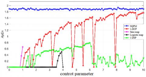
Figure 4. ApEn values: SQPM (b=c=0), 1-DCP, 1DSP (β=0.3306)

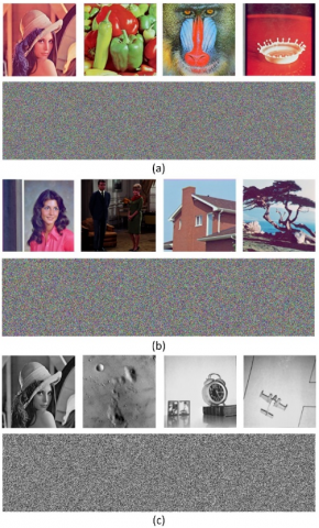
The security analysis of the proposed MIE algorithm was conducted on a PC equipped with 16 GB RAM and a 2.80 GHz Intel Core i7 processor, utilizing MATLAB 2020a. For the simulations, three distinct groups of images from the USC-SIPI image database [55] were employed. Group 1 comprises the color images “Lena”, “Peppers”, “Baboon”, and “Splash”, each of size 512×512. Group 2 includes color images “Female” (4.1.04.tiff), “Couple” (4.1.02.tiff), “House” (4.1.05.tiff), and “Tree” (4.1.06.tiff), all of size 256×256. Group 3 consists of four grayscale images, namely “Lena”, “Moon”, “Clock”, and “Airplane”, each with dimensions of 256×256. The encryption outcomes for these three groups of images are illustrated in Figure 7.

7.png

Figure 7. Input images and encrypted versions of a) Group 1 b) Group 2 c) Group 3

4.1 Keyspace and key sensitivity analysis

An MIE algorithm requires a keyspace of $2^{100}$ or larger to effectively resist exhaustive search attacks [56]. The proposed MIE scheme incorporates five secret keys: $Key$, $key_1$, $key _2$, $k e y_3$, and $k e y_4$. Key is the first 384-bit long secret key generated by the SHA- 384 hash value of the combined input images. The other keys are integral in calculating the control parameters and the initial value for the SQPM in the diffusion phase. The precisions for $k e y_1, k e y_2, k e y_3$, and $k e y_4$ are experimentally set to $10^{-14}, 10^{-14}, 10^{-14}$, and $10^{-14}$, respectively. Consequently, the total keyspace size is calculated as $2^{384} \times 10^{52} \cong 1.67 \times 2^{556}$, which far exceeds the minimum required keyspace. This substantial keyspace size underscores the robustness of the proposed MIE method against exhaustive search attacks. Table 1 provides a comparative analysis of the keyspace sizes between this study and other MIE algorithms, highlighting the superior performance of the proposed scheme.

Key sensitivity implies that even a minor alteration in any of the secret keys during the decryption phase results in the inability to correctly recover the input images. To assess this, six key sensitivity analyses were conducted, with modifications as detailed in Table 2. For each analysis, a slight change was made to one secret key, keeping the others unaltered. Two key sensitivity tests were performed for each image group, and the decryption outcomes are presented in Figure 8. The results clearly illustrate that any minor deviation in a secret key renders the decrypted images unrecognizable, thereby confirming the high sensitivity of the proposed technique to the secret keys.

Table 1. Keyspace comparison with other MIE algorithms

8.png

Figure 8. Decryption results. Group 1: a) Key’s first bit flipped b) Key’s last bit flipped, Group 2: c) $\begin{gathered}k e y_1+10^{-14} \text { d) } k e y_2-10^{-10}, \text { Group } 3: \text { e) } k e y_3+10^{-14} \text { f) } \\ key_4-10^{-14}\end{gathered}$

Table 2. Key sensitivity analysis parameters

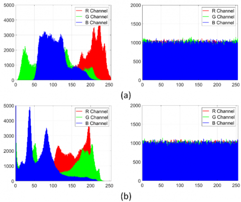
Histogram plots are a valuable tool for analyzing the pixel distribution in an image. Typically, the histogram plots of input images exhibit a non-uniform distribution, whereas encrypted images should display a uniform distribution to effectively resist statistical attacks. In the context of an MIE algorithm, particularly for color images, it is crucial that the histograms of the Red (R), Green (G), and Blue (B) channels across all images demonstrate uniform distribution. Figure 9 showcases the histogram graphs for both input and encrypted images in Group 1. As evidenced in the figure, the proposed MIE method successfully ensures a uniform pixel distribution across all channels of the encrypted images.

9a.png

9b.png

Figure 9. Histogram plots of input and encrypted images in Group 1: a) Lena b) Baboon c) Peppers d) Splash

The uniformity of a histogram graph can be quantitatively assessed by calculating its variance. The variance is computed using the following equation:

$\operatorname{var}=\frac{1}{256^2} \sum_{i=1}^{256} \sum_{j=1}^{256} \frac{\left(x_i-x_j\right)^2}{2}$             (19)

where, $x_i$ and $x_j$ represent the total numbers of the $i$-th and $j$ th pixels, respectively. To effectively resist statistical attacks, the histogram variance values of encrypted images should be substantially lower than those of the input images. This principle is exemplified in the proposed MIE algorithm, which demonstrates a significant reduction in the histogram variance values for the input images, as detailed in Table 3. For the tested input images, there is an average reduction in variance value by 99.9%. This substantial decrease in variance values strongly indicates the method’s capacity to resist statistical attacks.

Table 3. Histogram variance values

4.3 Correlation analysis

To evaluate resistance against statistical attacks, it is crucial to conduct correlation analysis in tandem with histogram analysis. Input images typically exhibit strong correlations between adjacent pixels in horizontal (H), vertical (V), and diagonal (D) directions. Additionally, in the case of color images, there exists a cross-channel correlation among the R, G, and B planes [57, 58]. A proficient MIE algorithm should effectively reduce both types of correlations to safeguard against potential statistical attacks. Figure 10 displays the distribution of adjacent pixels in the original and encrypted images from Group 3, along the horizontal, vertical, and diagonal directions. As evidenced in the figure, the proposed MIE algorithm successfully decorrelates the adjacent pixels in all three directions for all images. The correlation between neighboring pixels is quantified using a metric known as the correlation coefficient ($r_{a, b}$), which is defined in Eq. (20).

$r_{a, b}=\frac{\sum_{i=1}^K\left(a_i-E(a)\right)\left(b_i-E(b)\right)}{\sqrt{\sum_{i=1}^K\left(a_i-E(a)\right)^2} \sqrt{\sum_{i=1}^K\left(b_i-E(b)\right)^2}}$          (20)

where, $a_i$ and $b_i$ represent the values of adjacent pixels, while $K$ denotes the number of randomly selected pixel pairs. Additionally, $E(a)$ and $E(b)$ are the means of $a_i$ and $b_i$, respectively. For the purpose of calculating the correlation coefficient values, 10,000 unique pixel pairs were randomly chosen in all directions from both the tested input images and their corresponding encrypted images. The correlation coefficient values thus obtained are presented in Table 4. Notably, the correlation coefficients of the input images are close to 1, indicating a strong correlation. However, the coefficients for the encrypted images are very close to 0, signifying a successful disruption of the horizontal, vertical, and diagonal correlations between neighboring pixels. This disruption is consistently achieved across all channels of the input images by the proposed MIE algorithm.

Table 4. Correlation coefficient values

Table 5. Information entropy values

Figure 10. The distribution of adjacent pixels of the input and encrypted images in Group 3: a) Lena b) Moon c) Clock d) Airplane

Table 6. Information entropy (average) comparison

4.4 Information entropy analysis

In accordance with information theory, random systems inherently contain more information than deterministic systems. Consequently, the information entropy value of an encrypted image should exceed that of its corresponding input image. For a pixel represented by 8 bits, the information entropy (I) of a grayscale image or a single channel can be computed using the formula:

$I=\sum_{i=0}^{2^8-1} P\left(s_i\right) \frac{1}{\log _2 P\left(s_i\right)}$              (21)

where, $s_{i=0,1, . ., 255}$ is equal to the total number of pixels, and the values of $\mathrm{i}$ and $\mathrm{P}\left(\mathrm{s}_{\mathrm{i}}\right)$ can be calculated by dividing $s_i$ by the total number of pixels in an image. Theoretically, when the $I$ value is equal to 8 , a random image is obtained. An effective MIE method should yield encrypted images with information entropy values nearing this theoretical maximum. As shown in Table 5, the information entropy values of the encrypted images are greater than 7.99, indicating that the proposed MIE method successfully generates multiple random images/channels. Furthermore, Table 6 compares average information entropy values of the proposed method with several recent MIE algorithms for images of size $512 \times 512$. This comparison reveals that the proposed method exhibits similar or superior performance in terms of resisting information entropy attacks compared to other methods in the MIE literature.

4.5 Known-plaintext and chosen-plaintext attack analyses

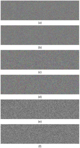
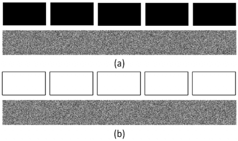
In scenarios involving known-plaintext attacks (KPAs) and chosen-plaintext attacks (CPAs), an attacker's primary objective is to decipher the secret keys. To counteract these types of attacks, the proposed MIE algorithm incorporates the SHA-384 hash value of the combined input images. Consequently, even if an attacker gains access to both the plaintext and ciphertext, they cannot derive meaningful information from the cryptosystem. The resistance of the proposed MIE method to KPAs and CPAs was evaluated by encrypting five all-black and five all-white images, each 100×200 in size, as illustrated in Figure 11. An attacker would be unable to extract any valuable information from the encrypted all-black or all-white images, as these encrypted outputs resemble noise-like, meaningless patterns.

11.png

Figure 11. Input images and encrypted versions. a) all-black b) all-white

4.6 Differential attack analysis

Differential attacks focus on uncovering details about the secret key or the plaintext image by analyzing the variations between the input and encrypted output images. For an MIE algorithm to be deemed resistant to differential attacks, it must exhibit a complete change in the output images when any pixel in the input images or channels is altered. To evaluate a cryptosystem's resilience against such attacks, metrics like the Number of Pixel Change Rate (NPCR) and Unified Average Changing Intensity (UACI) are utilized, as defined in the following equations:

$N P C R=\frac{1}{H \times W} \sum_{j=1}^W \sum_{i=1}^H D(i, j) \times 100 \%$             (22)

$U A C I=\frac{1}{H \times W} \sum_{j=1}^W \sum_{i=1}^H \frac{\left|E_1(i, j)-E_2(i, j)\right|}{255} \times 100 \%$                (23)

$D(i, j)= \begin{cases}1, & E_1(i, j) \neq E_2(i, j) \\ 0, & E_1(i, j)=E_2(i, j)\end{cases}$              (24)

where, $E_1$ and $E_2$ represent two ciphertext images derived from input images that are identical except for a single pixel variation. As demonstrated in Table 7, an arbitrary input image or channel is selected, and the value of a randomly chosen pixel is slightly altered. Remarkably, even a minor changesuch as increasing or decreasing the value of just one pixel in an input image-leads to significant alterations in a large proportion of pixels across all output images in the proposed method. The overall average values of the NPCR and UACI for the tested input images are $99.6002 \%$ and $33.4526 \%$, respectively. These averages closely align with the expected NPCR and UACI values of $99.61 \%$ and $33.46 \%$ [59], thereby confirming the proposed MIE technique's ability to resist differential attacks. Furthermore, Table 8 compares the average NPCR and UACI values of the proposed method with other state-of-the-art MIE algorithms. This comparison demonstrates that the proposed method performs comparably to the leading algorithms in the literature in terms of resisting differential attacks.

Table 7. NPCR and UACI values

Table 8. NPCR and UACI (average) comparison

4.7 Data loss and noise attack analysis

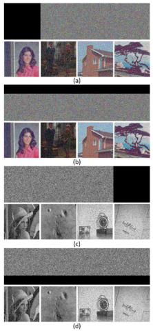
During the transmission of multiple images, it is possible that parts of the encrypted image might be cropped or the image could become contaminated with noise. In such scenarios, a robust MIE scheme should ensure that the decrypted images remain visually recognizable. For the images in Groups 2 and 3, decryption results are displayed in Figure 12, where it is assumed that 25% of the data is lost from different corners. The simulation results clearly demonstrate that the decrypted images are identifiable, despite the data loss. Additionally, to simulate potential noise attacks, salt and pepper noise (SPN) with densities of 0.1 and 0.3 is added to the encrypted images across all groups. As evidenced in Figure 13, all decrypted images remain recognizable, though the amount of visual information diminishes with increasing noise density. Consequently, these results affirm that the proposed MIE algorithm is capable of effectively resisting both data loss and noise attacks.

12.png

Figure 12. Data loss analysis. a), b) 25% data loss for images in group 2. c), d) 25% data loss for images in group 3

13.png

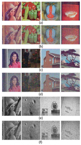
Figure 13. Noise attack analysis. a), b) 0.1 and 0.3 SPN for images in group 1. c), d) 0.1 and 0.3 SPN for images in group 2. e), f) 0.1 and 0.3 SPN for images in group 3

4.8 Encryption and decryption time analysis

Table 9. Encryption and decryption times (in seconds)

The suitability of an MIE algorithm for real-time applications can be gauged by assessing the time it takes for encryption and decryption. Table 9 presents the average encryption and decryption times recorded for the proposed method when applied to the tested images. Additionally, Table 10 compares the encryption times of this work with those of various other MIE algorithms. It is important to note that encryption time is influenced not only by the algorithm itself but also by the hardware and software specifications, which are duly listed in the table for a comprehensive understanding. The proposed MIE algorithm demonstrates relatively rapid performance, capable of encrypting four color images of size 512×512 in approximately 0.56 seconds. Hence, its speed makes it a potentially attractive option for real-time applications.

4.9 Future work

The MIE algorithm introduced in this study is designed to encrypt images of identical sizes. Furthermore, it requires that all images within a group be of the same type, either all grayscale or all color. Future research endeavors will focus on developing new algorithms capable of encrypting images of varying types and sizes within a single group, thereby enhancing versatility and applicability.

Table 10. Encryption time (in seconds) comparison