Ahmet Haydar Ornek*![]() | Murat Ceylan
| Murat Ceylan![]()
© 2024 The authors. This article is published by IIETA and is licensed under the CC BY 4.0 license (http://creativecommons.org/licenses/by/4.0/).
OPEN ACCESS
Deep learning models are proficient at predicting target classes, but they need to explain their predictions. Explainable Artificial Intelligence (XAI) offers a promising solution by providing both transparency and object detection capabilities to classification models. Mask detection plays a crucial role in ensuring the safety and well-being of individuals by preventing the spread of infectious diseases. A new visual XAI method called HayCAM+ is proposed to address the limitations of the previous method known as HayCAM, such as the need to select the number of filters as a hyper-parameter and the use of fully-connected layers. When object detection is performed using activation maps created via various methods, including GradCAM, EigenCAM, GradCAM++, LayerCAM, HayCAM, and HayCAM+, it is found that HayCAM+ provides the best results with an IoU score of 0.3740 (GradCAM: 0.1922, GradCAM++: 0.2472, EigenCAM: 0.3386, LayerCAM: 0.2476, HayCAM: 0.3487) and a Dice score of 0.5376 (GradCAM: 0.3153, GradCAM++: 0.3923, EigenCAM: 0.5003, LayerCAM: 0.3928, HayCAM: 0.5098). By using dynamical dimension reduction to eliminate unrelated filters in the last convolutional layer, HayCAM+ generates more focused activation maps. The results demonstrate that HayCAM+ is an advanced activation map method for explaining decisions and detecting objects using deep classification models.
class activation mapping, deep learning, explainable artificial intelligence, HayCAM, visual explanation, weakly-supervised object detection
Research in the field of Artificial Intelligence (AI) has shown that it is capable of successfully solving image-based tasks, such as image classification, in various industries, including medicine [1-3], retail [4-6], and personal protective equipment [7-9]. This capability arises from researchers’ ability to train deep model architectures without overfitting [10]. However, despite their success, the decisions made by deep models are only partially explained due to their non-linear nature. The field of research focused on understanding how AI models make decisions is known as Explainable Artificial Intelligence (XAI) [11].
Figure 1. The general problems of the GradCAM. While GradCAM generates scattered activation maps, HayCAM+ generates focused activation maps
To address the lack of explanation in deep models, we propose a new visual XAI method called HayCAM+. Deep models consist of convolution, pooling, activation function, and normalization layers, which enable them to learn representations [12]. Although these layers allow for the combination of different features, the non-linear nature of these layers means that the explanation side of deep models is decreased, resulting in them being referred to as “Black Box” models [13]. Figure 1 illustrates the general problem of deep models and the developed solutions. As shown at the top of Figure 1, deep models can accurately predict classes, but they cannot explain their decisions (a.k.a., Black-Box models).
The goal of XAI is to provide understandable explanations for the decisions made by AI models, which builds trust between the models and experts, such as developers, doctors, and engineers [14, 15]. With XAI, experts can understand why a particular decision was made, how the model learned, which parts of the content were emphasized, and what factors contributed to the classification. For example, when an image is fed into a classification model, the experts can only understand how the model predicted using XAI. By providing transparent, understandable explanations, XAI addresses the inherent "black box" nature of complex AI models. This transparency fosters trust between medical professionals and AI systems, as doctors can confidently rely on and validate the decisions made by these models.
XAI methods are typically divided into three categories: visual, numerical, and rule-based methods [16]. Numerical methods calculate the importance of input features by adding or removing them, while rule-based methods create a decision tree structure [17]. Visual methods, on the other hand, reveal which parts of an image are relevant to the model’s decision [18]. Given the thousands of parameters in a deep model, numerical and rule-based methods are better suited for explaining the decisions made by these models. However, visual methods are ideal for explaining decisions by identifying the most essential parts of an image [19, 20]. As illustrated in Figure 1, activation maps are generated to reveal which parts of an image are related to the decision.
In our previous work, we proposed HayCAM [21] as a visual XAI method and compared it to other well-known methods such as GradCAM [22], EigenCAM [23], and GradCAM++ [24]. Our primary contribution was to reduce the last layer of the deep model during visualization to ignore irrelevant filters and obtain a more focused activation map.
HayCAM+ builds on HayCAM by addressing its primary limitations: (i) the number of components was manually selected, and (ii) the fully connected layer weighted reduced layers. As an advanced visual XAI method, HayCAM+ is simpler and more effective than other methods, such as GradCAM, EigenCAM, GradCAM++, LayerCAM, and HayCAM.
Our main contributions in proposing HayCAM+ are as follows: (i) the number of PCA components is dynamically calculated, (ii) Weight dependency in fully-connected layer is removed, and (iii) LayerCAM is added as a new method to compare.
Section 1 introduces the current state and advancements in Artificial Intelligence, as well as the need for Explainable Artificial Intelligence (XAI). Section 2 discusses related XAI methods across various domains, such as medicine, retail, and personal protective equipment. Section 3 provides details about the materials and methods used in the study. Section 4 introduces the proposed method, HayCAM+, and explains how it overcomes the limitations of the previous method, HayCAM. Section 5 describes the experiments and results obtained using HayCAM+ and compares them with other XAI methods, such as GradCAM, EigenCAM, GradCAM++, LayerCAM, and HayCAM. Section 6 discusses the achieved results, their implications, and limitations. Finally, Section 7 provides the study's conclusion, including the significance of the proposed method and its future potential.
Numerical explanations involve calculating the contribution of input features to decision-making by training the AI model with different numbers of features and observing the resulting performance [25]. Rule-based methods are another approach to building explanations by creating decision rules from input features to decisions. These methods can improve the model’s performance while retaining explanations, but there is often a trade-off between performance and explanation quality. Given the large number of inputs in a simple deep model, it is difficult to determine the importance of each feature.
Visual methods are another approach to explaining deep Convolutional Neural Networks (CNNs), by identifying the most essential parts of the content. One standard method is to visualize the convolution filters and layers to understand whether the model is learning effectively [26]. If the layers reveal unrelated parts to the desired classes, it may indicate overfitting or other issues that require further exploration.
Perturbation-based methods [27, 28] involve windowing the input content with different shapes to measure the output. Local Interpretable Model-Agnostic (LIME) approach creates linear models by dividing decisions into smaller parts. Similarly, the Shapley Additive Explanations approach utilizes non-linear models for the same purpose.
Deconvolution Networks [29] create hierarchical visualizations by propagating from the last layers to the first layers. Class Activation Mapping (CAM) [30] is a method that uncovers the contributions of pixels using the last convolutional layer. However, CAM requires removing the fully-connected layer and adding Global Average Pooling, which can reduce performance [31]. Gradient-based CAMs (GradCAMs) do not have these limitations and can be applied without modifying the model.
GradCAM-based methods, such as GradCAM++, take class information into account to generate activations separately for each class. GradCAM++ utilizes second-order gradients in the last convolutional layer of deep models to generate activations when compared to GradCAM. In contrast, LayerCAM provides activation mapping using various layers of the deep models, while EigenCAM reduces the last layer using Singular Value Decomposition (SVD) to generate a focused activation map. However, EigenCAM directly decreases the convolutional layer to one filter without measuring the importance of filters in the layer. HayCAM+ utilizes Principal Component Analysis (PCA) to measure the importance of filters and generate more focused activation mapping. This approach calculates the number of PCA components dynamically and removes weight dependency in the fully-connected layer. Since the other methods use all of the filters in the last convolutional layer, they cause more scattered areas over the images. HayCAM+, as a new method, reduces the filters and creates more focused areas.
In this section, the materials and methods used in the study are presented in detail. The proposed HayCAM+ method is also described. The experiments and results are presented in this section as well.
3.1 Material
In this study, mask images were obtained from open-source and custom images to create a dataset of 23,140 images for training, validation, and testing. The experiments were conducted on a Centos 7 Linux server with a Tesla GPU. The Python programming language was used along with the PyTorch framework for deep learning operations and OpenCV for computer vision tasks. Further details can be found in the authors' previous work [32].
3.2 Classification of the images
Image classification is a basic process in computer vision that aims to determine the category of an image when it is fed into a model. Feature engineering and classification are necessary to obtain class information [33]. The process of feature engineering involves two main steps: feature extraction and feature selection.
Features encompass any relevant information that can be derived from an image, such as edges, circles, patterns, colors, and areas, among others. Feature extraction methods, like the Canny Edge Detector [34] and Histograms of the Oriented Gradients [35], extract these features. After extracting the features, their dimensions are reduced using feature selection methods like Singular Value Decomposition (SVD) [36]. This reduction is necessary because the high dimensionality of the features can lead to information noise, increased time costs, and higher processing costs for the classification methods.
Once the features have been reduced in dimensionality, classification methods like Artificial Neural Networks (ANN) [37] and Support Vector Machines (SVM) [38] are utilized to classify the features and obtain class information. However, a significant limitation of machine learning methods is that feature engineering needs to be carried out manually.
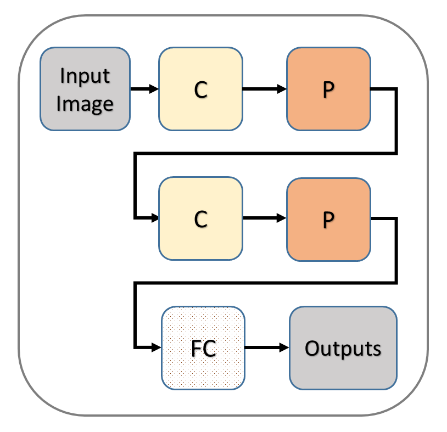
Deep learning methods, such as CNNs, address this limitation by automatically performing both feature engineering and classification through the use of operations and layers such as convolution, pooling, and fully-connected layers. A CNN model can be visualized as shown in Figure 2.
Figure 2. A basic CNN model. C, P, and FC stand for Convolution, Pooling and Fully-Connected respectively. When C and P are frozen it is called basic transfer learning
As shown in Figure 2, a simple CNN model consists of a combination of convolution, pooling, and fully-connected layers. For instance, a CNN model can have a structure of 3 convolution layers, two pooling layers, and two fully-connected layers, or five convolution layers, five pooling layers, and three fully-connected layers. Convolutional layers automatically extract features from images, while pooling layers reduce the dimensionality of the extracted features. Finally, the fully-connected layer classifies the reduced features to obtain class information. In this study, a CNN model is utilized to classify images into “mask” and “no mask” classes.
While CNN models are effective at image classification, they contain thousands of parameters that result in high operational costs. To reduce costs and maintain high performance, transfer learning is employed [39-42]. The basic idea of transfer learning is that the same convolutional weights, which capture low-level information such as edges, can be shared among CNN models. For example, some pre-trained models like ResNet [43], VGG [44], and Inception [45] are trained on the ImageNet dataset, which consists of images classified into 1000 different classes. Since the first layers of these pre-trained models capture low-level features, they can be utilized in custom models. Figure 3 displays a basic ResNet18 model.
Figure 3. A Resnet model. (3, 64) shows 64 times 3×3 convolution and (3,512) shows 512 times 3×3 convolution. The arrows point to skip connections. GAP and FCL stand for Global Average Pooing and Fully-Connected Layer respectively
In this particular study, the pre-trained ResNet18 model is chosen and adapted to the mask dataset for comparison with the HayCAM approach. ResNet18 is one of the state-of-the-art deep learning models that has been shown to outperform other popular models like VGG16 in terms of accuracy and efficiency. It can train a high-quality model with a low amount of data, making it well-suited for devices. The modified ResNet18 model is then trained on the dataset.
As depicted in Figure 3, ResNet18 comprises convolutional layers, pooling layers, global average pooling, fully-connected layers, and skip connections. Skip connections help to alleviate the overfitting issue by allowing gradients to flow from the last layers to the earlier ones.
3.3 Class activation mapping methods
CAM methods aim to explain the decisions made by CNNs by visualizing their last convolutional layers through various approaches such as GradCAM, EigenCAM, GradCAM++, LayerCAM [46], and HayCAM. The first CAM method, as described by Eq. (1), only requires the Global Average Pooling (GAP) layer (as shown in Eq. (2)) after the last convolutional layer, which results in a decrease in performance since the fully-connected layer is removed.
$L=\sum_p w_p A^p$ (1)
$G A P_p=\frac{1}{N} \sum_i \sum_j A_{i j}^p$ (2)
where, L is the created importance map, wp is the weights importance of the layers and Ap is the last convolutional layer. GradCAM (Eq. (3)) that is generalization of the CAM, removes the limitations such that fully-connected layer can be used in the CNN architecture. GradCAM uses the gradients of the classes propagating from the last convolutional layer.
$w_{p(\operatorname{GradCAM})}=\frac{1}{N} \sum_j \sum_k \frac{\partial Y}{\partial A_{j k}^p}$ (3)
In GradCAM, the weights importance of the layers for the last convolutional layer is denoted by wp(GradCAM), while Y represents the desired class. The importance map is created using Eq. (1) with the wp(GradCAM) values. GradCAM++ is another method used to identify important regions in an image. In addition to calculating first-order gradients, it also computes second-order derivatives and applies a ReLU function to eliminate negative values. The weights of GradCAM++ are determined using Eq. (4).
$w_{p(G r a d C A M++)}=\sum_j \sum_k \alpha_{j k}^p \operatorname{ReLU}\left(\frac{\partial Y}{\partial A_{j k}^p}\right)$ (4)
LayerCAM generates importance maps by combining multiple convolutional layers, not just the last one. This is achieved by using the second-order derivatives. The weighting of the layers is determined by eliminating any negative values.
$L_{LaverCAM}=\operatorname{ReLU}\left(\sum_p A^p\right)$ (5)
EigenCAM, as shown in Eq. (6), applies SVD (as described in Eq. (7)) to find the first principal component of the GradCAM methods. This results in a decrease in the size of the last convolutional layer from (512, 7×7) to (1, 7×7).
$L_{EigenCAM}=A^p V_1$ (6)
$A^p=U E V^t$ (7)
where, V and U are orthogonal matrices, and E is a diagonal matrix. V, U, and E are known right singular vectors, left singular vectors, and singular values respectively. The first element V1 of the V is used to get the EigenCAM importance map. HayCAM reduces the last convolutional layer and related weights (Eq. (8)) by PCA, and creates the activation mapping (Eq. (9)).
$w_{p(\text { HayCAM })}, A_{(\text {HayCAM })}^p=P C A\left(\frac{1}{N} \sum_j \sum_k \frac{\partial Y}{\partial A_{j k}^p}, A^p\right)$ (8)
$L_{\text {HayCAM }}=\sum_p w_{p(\text { HayCAM })} A_{(\operatorname{HayCAM})}^p$ (9)
3.4 Calculating the number of filters dynamically
Data in the real world often comprises both related and unrelated features. Dimension reduction techniques aim to minimize the unrelated features as much as possible. Principal Component Analysis (PCA) has been used as a dimension reduction method for decades and is mainly employed to calculate the importance of features by computing eigenvalues.
PCA generates a covariance matrix to obtain eigenvalues and eigenvectors. The importance of each eigenvector is determined by its corresponding eigenvalue. After sorting the eigenvectors by eigenvalues, the first “n” elements are selected as principal eigenvectors. The value of “n” can be chosen manually, as is the case in HayCAM. For further information, please refer to the study of Örnek and Ceylan [21].
|
Algorithm 1. Calculating number of filters dynamically |
|
|
|
|
|
|
This study dynamically calculates the value of "n" by using the variance of the sorted eigenvectors. The process for selecting the appropriate number of filters is outlined in Algorithm 1, and it is as follows: (i) the variance for each sorted eigenvector is computed, (ii) the obtained variances are summed, (iii) each variance is divided by the summed variance, (iv) the divided variances are then summed from the first to the "n"th element until the summed variance is higher than 0.9. This means that if the selected eigenvectors account for 90% of the variance, it is sufficient to select these as the principal eigenvectors.
3.5 Evaluation of the bounding boxing
A bounding box is defined by four components: x, y, w, and h, which are associated with an object. Here, (x, y) refers to the top left corner of the bounding box, w refers to the width of the box, and h refers to the height of the box. Figure 4 provides a visual representation of these components. This information is taken from the study of Zhao et al. [47].
Figure 4. A sample bounding box intersection and union
In Figure 4, the ground truth bounding box is represented by a solid line, while the estimated bounding box is represented by dashed lines. The Intersection over Union (IoU) metric (Eq. (10)) and Dice coefficient (Eq. (11)) are used to evaluate how well the estimated bounding box aligns with the ground truth bounding box. Both IoU and Dice scores range between 0 and 1, with scores closer to 1 indicating a better alignment between the ground truth and estimated bounding boxes. Both IoU and Dice are commonly used object detection indicators and can intuitively reflect the performance of the model [48, 49]. Secondly, the calculation process of IoU and Dice is relatively simple and easy to implement and calculate.
$I o U=\frac{|B o x 1| \cap|B o \times 2|}{|B o x 1| \cup B o \times 2 \mid}$ (10)
Dice $=\frac{2 *(\mid \text { Box } 1|\cap| \text { Box } 2 \mid)}{\mid \text { Box1 } 1|+| \text { Box } 2 \mid}$ (11)
HayCAM+ is a novel visual XAI method that aims to create more focused activation maps by selecting important filters in the last convolutional layer. To achieve this, HayCAM+ reduces only the last convolutional layer (Eq. (12)) using PCA, without taking weights into account. The number of PCA components is dynamically calculated, as described in the previous section. Once the PCA components are obtained, they are summed to obtain the HayCAM+ activation mapping (Eq. (13)). This method enables HayCAM+ to create more focused activation maps that highlight the most important features in the input data. Algorithm 2 outlines the steps involved in the HayCAM+ method.
$A_{(\text {HayCAM+) }}^p=P C A\left(A^p\right)$ (12)
$L_{\text {HayCAM+ }}=\sum_p A_{(\mathrm{HayCAM}+)}^p$ (13)
|
Algorithm 2. HayCAM+ (proposed) |
|
|
|
|
|
|
First, the model is used to infer the activations in the last convolutional layer, which contains 512 filters of size 7×7. The filters are then reshaped to 512×49 to enable vector operations such as subtraction. The mean of the filters is subtracted to center them. Next, PCA is used to obtain the main filters by selecting the first n elements (i.e., n elements that have 90% variance) after sorting the eigenvectors according to eigenvalues. This step removes unrelated or noisy filters from the last convolutional layer, leaving only the class-related information. The values of the selected filters are then summed to obtain a single filter, which represents the HayCAM+ activation map. The resulting (1×49) filter is reshaped to (7×7) as seen in Figure 5 and resized to (224×224) to highlight the input image.
By applying the changes, HayCAM+ achieves better performance by its IoU score of 0.3740 (GradCAM 0.1922, GradCAM++ 0.2472, EigenCAM 0.3386, LayerCAM 0.2476, and HayCAM 0.3487) and a Dice score of 0.5376 (GradCAM 0.3153, GradCAM++ 0.3923, EigenCAM 0.5003, LayerCAM 0.3928, and HayCAM 0.5098). This performance is attributed to HayCAM+'s utilization of dynamic dimension reduction, eliminating irrelevant filters in the last convolutional layer, thereby producing activation maps enhanced focus and precision.
Figure 5. Sample 7×7 activation mapping images
The pre-trained ResNet18 classifier model is used for the study, which was modified by removing the 1000-class fully-connected layer and adding a new fully-connected layer with only 2 classes: “mask” and “no mask”. The model was trained on a dataset of 18,400 training images and 200 validation images, and then tested on 4,540 images.
The results showed that the ResNet18 model achieved a 4.42% loss in classifying images into the “mask” and “no mask” categories. However, to better understand how the model works and which regions it considers important for classification, the researchers used several visual explainability methods, including GradCAM, EigenCAM, GradCAM++, LayerCAM, HayCAM, and HayCAM+. These methods aim to highlight the important areas of an image that are related to the predicted class. The resulting activation maps and their combination with the input images are shown in Figures 6 and 7.
Figures 6 and 7 show that all of the methods can identify important areas in the input images, but some methods create less focused areas than others. The results suggest that a classifier model can also function as an object detector model.
HayCAM+ produces the most focused areas, as shown in Figure 8. A comprehensive evaluation can be found in Table 1, focusing on Intersection over Union (IoU) values, and Table 2, focusing on Dice values, the superior performance of the HayCAM+ method.
Since PCA is employed to reduce the dimensionality of the feature space, it helps in simplifying the complexity of the data representation while retaining the most significant features. By selecting the first n elements (eigenvectors) that collectively account for 90% of the variance, the dimensionality is effectively reduced, focusing on the most informative aspects of the data. Sorting the eigenvectors according to eigenvalues allows for the identification of the most critical filters in the last convolutional layer. This is advantageous because it effectively filters out unrelated or noisy filters. These unrelated filters may capture irrelevant patterns or noise, which, when removed, streamlines the subsequent analysis, ensuring that the retained filters carry more pertinent information related to the target classes. Therefore, HayCAM+ encapsulates the critical class-related information while excluding extraneous details. It serves as a concise and focused representation of the features influencing the model's decision, contributing to improved interpretability.
Figure 6. Generated activation maps
Figure 7. The combination of activation maps and input images
Figure 8. Object detection results
Table 1. The IoU results
|
Image no |
GradCAM |
GradCAM++ |
EigenCAM |
LayerCAM |
HayCAM |
HayCAM+ |
|
a1 |
0.0523 |
0.1214 |
0.1784 |
0.1214 |
0.2828 |
0.3156 |
|
a2 |
0.0499 |
0.1188 |
0.1647 |
0.1188 |
0.2816 |
0.2895 |
|
a3 |
0.0835 |
0.1488 |
0.2087 |
0.1488 |
0.4269 |
0.4782 |
|
a4 |
0.1162 |
0.1752 |
0.2457 |
0.1752 |
0.3024 |
0.3105 |
|
a5 |
0.1014 |
0.1900 |
0.2685 |
0.1881 |
0.2699 |
0.2706 |
|
a6 |
0.1146 |
0.1345 |
0.1879 |
0.1358 |
0.3337 |
0.3568 |
|
… |
|
|
|
|
|
|
|
a154 |
0.1285 |
0.1534 |
0.2131 |
0.1519 |
0.4179 |
0.4575 |
|
a155 |
0.2039 |
0.2555 |
0.3397 |
0.2555 |
0.3460 |
0.3948 |
|
a156 |
0.2275 |
0.2803 |
0.3643 |
0.2830 |
0.3735 |
0.4205 |
|
a157 |
0.2329 |
0.2866 |
0.3593 |
0.2893 |
0.4017 |
0.4231 |
|
a158 |
0.1205 |
0.1484 |
0.2018 |
0.1469 |
0.2845 |
0.2905 |
|
a159 |
0.1293 |
0.1550 |
0.2129 |
0.1534 |
0.3199 |
0.4132 |
|
a160 |
0.1486 |
0.1898 |
0.3104 |
0.1916 |
0.3468 |
0.4039 |
|
Average |
0.1922 |
0.2472 |
0.3386 |
0.2476 |
0.3487 |
0.3740 |
Table 2. The dice results
|
Image no |
GradCAM |
GradCAM++ |
EigenCAM |
LayerCAM |
HayCAM |
HayCAM+ |
|
a1 |
0.0994 |
0.2165 |
0.3029 |
0.2165 |
0.4409 |
0.4798 |
|
a2 |
0.0951 |
0.2123 |
0.2828 |
0.2123 |
0.4395 |
0.4490 |
|
a3 |
0.1542 |
0.2148 |
0.2941 |
0.2129 |
0.2924 |
0.2903 |
|
a4 |
0.2082 |
0.2983 |
0.3945 |
0.2983 |
0.4644 |
0.4738 |
|
a5 |
0.1842 |
0.3193 |
0.4233 |
0.3166 |
0.4251 |
0.4260 |
|
a6 |
0.2056 |
0.2371 |
0.3164 |
0.2391 |
0.5004 |
0.5260 |
|
… |
|
|
|
|
|
|
|
a154 |
0.2278 |
0.2660 |
0.3513 |
0.2637 |
0.5895 |
0.6278 |
|
a155 |
0.3388 |
0.4070 |
0.5072 |
0.4070 |
0.5141 |
0.5661 |
|
a156 |
0.3707 |
0.4379 |
0.5341 |
0.4411 |
0.5438 |
0.5921 |
|
a157 |
0.3778 |
0.4455 |
0.5286 |
0.4487 |
0.5731 |
0.5946 |
|
a158 |
0.2151 |
0.2584 |
0.3358 |
0.2562 |
0.4430 |
0.4502 |
|
a159 |
0.2290 |
0.2683 |
0.3510 |
0.2660 |
0.4847 |
0.5847 |
|
a160 |
0.2588 |
0.3190 |
0.4738 |
0.3215 |
0.5150 |
0.5754 |
|
Average |
0.3153 |
0.3923 |
0.5003 |
0.3928 |
0.5098 |
0.5376 |
According to the results shown in Figure 8, HayCAM+ produces the most precise areas of interest, and it also has the highest IoU and Dice values. This implies that HayCAM+ is the best approach for both explaining decisions and identifying objects in input images.
The field of computer vision heavily relies on image classification, and CNNs are widely used for this purpose. While CNNs achieve high classification accuracy, their non-linear nature makes them difficult to explain. To address this challenge, various visual methods such as GradCAM, EigenCAM, and HayCAM have been developed to provide insights into what a CNN learns. In this study, a new visual method called HayCAM+ is proposed not only to explain what a CNN learns but also to generate more focused activation maps.
Figure 7 demonstrates that all the methods can identify important regions in the images, but HayCAM+ produces the most focused areas, indicating that a classifier model can not only classify images but also locate class objects. Figure 8 displays the detected mask images with bounding boxes and IoU values. More focused areas lead to better object detection performance, as indicated in Table 1 and Table 2. It is evident that HayCAM+ outperforms the other methods with IoU and Dice scores of 0.3710 and 0.5376, respectively.
HayCAM+ uses the last convolutional layers of the CNN. It would be interesting to explore the possibility of using different layers of the CNN for various datasets. This could potentially lead to even more accurate and efficient results, as different layers may be better suited for different types of images or data.
Deep learning models, particularly CNNs, have become popular for their ability to achieve high classification accuracy in various tasks. However, their complex architecture and vast number of parameters make it difficult to interpret how they make decisions. As a result, there is a need to develop techniques that can explain the reasoning behind the model’s decisions and highlight the important features that lead to the classification result. This is especially important in applications where transparency and interpretability are critical, such as medical diagnosis, autonomous driving, and fraud detection. HayCAM+ can be used in these areas. In the field of medical imaging, HayCAM+ could be instrumental in enhancing the interpretability of deep learning models used for diagnostic purposes. HayCAM+ can be applied to improve object recognition and localization tasks. Its ability to produce more focused activation maps allows for better localization of objects within images, contributing to the development of more accurate and reliable computer vision systems. HayCAM+ may find utility in the development of computer vision systems for autonomous vehicles. The enhanced interpretability and focused activation maps can aid in understanding the driving decisions made by AI models, making them more transparent and trustworthy for safe navigation. In industrial settings, particularly in quality control processes, HayCAM+ might be applied to enhance the inspection of manufactured products. By providing clearer insights into the features contributing to classification decisions, it can contribute to the improvement of product quality assessment. HayCAM+ could play a role in augmented reality applications by facilitating more accurate and contextually relevant virtual object placement. The focused activation maps can aid in aligning virtual elements with real-world objects, enhancing the overall user experience. HayCAM+ might be incorporated into systems that involve human-computer interaction, such as gesture recognition or facial expression analysis. The focused activation maps can contribute to more precise identification of relevant facial features or gestures, improving the accuracy of interaction models.
We introduce a novel visual Explainable AI (XAI) method called HayCAM+ that generates the most focused areas compared to other XAI methods. These areas aid in object detection and demonstrate that a classifier model can not only classify images but also highlight important regions and detect objects. The findings suggest that there are still open areas in basic processes like classification that need to be uncovered and explained to establish trust between AI machines and humans. Since almost all models need an explanation, HayCAM+ can be applied to different datasets.
In future studies, our aim is to delve deeper into the world of XAI by exploring and developing novel XAI methods that not only provide more accurate explanations but also enable us to gain a deeper understanding of the underlying mechanisms of deep learning models. We are considering the incorporation of attention mechanisms to further refine the interpretability of deep learning models. Investigating methods for dynamically assessing feature importance during different stages of model inference. Exploring techniques for quantifying uncertainty in model predictions. Considering the development of interactive XAI methods that allow users, such as domain experts or end-users, to actively query the model for specific explanations.
This work was supported by Huawei Türkiye R&D Center.
[1] Hamet, P., Tremblay, J. (2017). Artificial intelligence in medicine. Metabolism, 69: S36-S40. https://doi.org/10.1016/j.metabol.2017.01.011
[2] Rajpurkar, P., Chen, E., Banerjee, O., Topol, E.J. (2022). AI in health and medicine. Nature Medicine, 28(1): 31-38. https://doi.org/10.1038/s41591-021-01614-0
[3] He, J., Baxter, S.L., Xu, J., Xu, J., Zhou, X., Zhang, K. (2019). The practical implementation of artificial intelligence technologies in medicine. Nature Medicine, 25(1): 30-36. https://doi.org/10.1038/s41591-018-0307-0
[4] Semenov, V.P., Chernokulsky, V.V., Razmochaeva, N.V. (2017). Research of artificial intelligence in the retail management problems. In 2017 IEEE II International Conference on Control in Technical Systems (CTS), St. Petersburg, Russia, pp. 333-336. https://doi.org/10.1109/CTSYS.2017.8109560
[5] Moore, S., Bulmer, S., Elms, J. (2022). The social significance of AI in retail on customer experience and shopping practices. Journal of Retailing and Consumer Services, 64: 102755. https://doi.org/10.1016/j.jretconser.2021.102755
[6] Pillai, R., Sivathanu, B., Dwivedi, Y.K. (2020). Shopping intention at AI-powered automated retail stores (AIPARS). Journal of Retailing and Consumer Services, 57: 102207. https://doi.org/10.1016/j.jretconser.2020.102207
[7] Sánchez, S.M., Lecumberri, F., Sati, V., Arora, A., Shoeibi, N., Rodríguez, S., Rodríguez, J.M.C. (2020). Edge computing driven smart personal protective system deployed on NVIDIA Jetson and integrated with ROS. In Highlights in Practical Applications of Agents, Multi-Agent Systems, and Trust-worthiness. The PAAMS Collection: International Workshops of PAAMS 2020, L'Aquila, Italy, pp. 385-393. https://doi.org/10.1007/978-3-030-51999-5_32
[8] Vukicevic, A.M., Djapan, M., Isailovic, V., Milasinovic, D., Savkovic, M., Milosevic, P. (2022). Generic compliance of industrial PPE by using deep learning techniques. Safety Science, 148: 105646. https://doi.org/10.1016/j.ssci.2021.105646
[9] Balakreshnan, B., Richards, G., Nanda, G., Mao, H., Athinarayanan, R., Zaccaria, J. (2020). PPE compliance detection using artificial intelligence in learning factories. Procedia Manufacturing, 45: 277-282. https://doi.org/10.1016/j.promfg.2020.04.017
[10] Theckedath, D., Sedamkar, R.R. (2020). Detecting affect states using VGG16, ResNet50 and SE-ResNet50 networks. SN Computer Science, 1: 1-7. https://doi.org/10.1007/s42979-020-0114-9
[11] Arrieta, A.B., Díaz-Rodríguez, N., Del Ser, J., Bennetot, A., Tabik, S., Barbado, A., Tabik, S., Barbado, A., Garcia, S., Gil-Lopez, S., Molina, D., Benjamins, R., Chatila, R., Herrera, F. (2020). Explainable Artificial Intelligence (XAI): Concepts, taxonomies, opportunities and challenges toward responsible AI. Information Fusion, 58: 82-115. https://doi.org/10.1016/j.inffus.2019.12.012
[12] Krizhevsky, A., Sutskever, I., Hinton, G.E. (2012). Imagenet classification with deep convolutional neural networks. Advances in Neural Information Processing Systems, 25.
[13] Confalonieri, R., Weyde, T., Besold, T.R., del Prado Martín, F.M. (2021). Using ontologies to enhance human understandability of global post-hoc explanations of black-box models. Artificial Intelligence, 296: 103471. https://doi.org/10.1016/j.artint.2021.103471
[14] Xu, F., Uszkoreit, H., Du, Y., Fan, W., Zhao, D., Zhu, J. (2019). Explainable AI: A brief survey on history, research areas, approaches and challenges. In Natural Language Processing and Chinese Computing: 8th CCF International Conference, NLPCC 2019, Dunhuang, China, pp. 563-574. https://doi.org/10.1007/978-3-030-32236-6_51
[15] Gade, K., Geyik, S.C., Kenthapadi, K., Mithal, V., Taly, A. (2019). Explainable AI in industry. In Proceedings of the 25th ACM SIGKDD International Conference on Knowledge Discovery & Data Mining, pp. 3203-3204. https://doi.org/10.1145/3292500.3332281
[16] Recio-García, J.A., Díaz-Agudo, B., Pino-Castilla, V. (2020). CBR-LIME: A case-based reasoning approach to provide specific local interpretable model-agnostic explanations. In Case-Based Reasoning Research and Development: 28th International Conference, ICCBR 2020, Salamanca, Spain, pp. 179-194. https://doi.org/10.1007/978-3-030-58342-2_12
[17] Mahbooba, B., Timilsina, M., Sahal, R., Serrano, M. (2021). Explainable artificial intelligence (XAI) to enhance trust management in intrusion detection systems using decision tree model. Complexity, 2021: 6634811. https://doi.org/10.1155/2021/6634811
[18] Došilović, F.K., Brčić, M., Hlupić, N. (2018). Explainable artificial intelligence: A survey. In 2018 41st International Convention on Information and Communication Technology, Electronics and Microelectronics (MIPRO), Opatija, Croatia, pp. 0210-0215. https://doi.org/10.23919/MIPRO.2018.8400040
[19] Fidel, G., Bitton, R., Shabtai, A. (2020). When explainability meets adversarial learning: Detecting adversarial examples using SHAP signatures. In 2020 International Joint Conference on Neural Networks (IJCNN), Glasgow, UK, pp. 1-8. https://doi.org/10.1109/IJCNN48605.2020.9207637
[20] Hase, P., Bansal, M. (2020). Evaluating explainable AI: Which algorithmic explanations help users predict model behavior? arXiv preprint arXiv:2005.01831. https://arxiv.org/abs/2005.01831
[21] Örnek, A.H., Ceylan, M. (2022). HayCAM: A novel visual explanation for deep convolutional neural networks. Traitement du Signal, 39(5): 1711-1719. https://doi.org/10.18280/ts.390529
[22] Selvaraju, R.R., Cogswell, M., Das, A., Vedantam, R., Parikh, D., Batra, D. (2017). Grad-cam: Visual explanations from deep networks via gradient-based localization. In Proceedings of the IEEE International Conference on Computer Vision, Venice, Italy, pp. 618-626. https://doi.org/10.1109/ICCV.2017.74
[23] Muhammad, M.B., Yeasin, M. (2020). Eigen-cam: Class activation map using principal components. In 2020 International Joint Conference on Neural Networks (IJCNN), Glasgow, UK, pp. 1-7. https://doi.org/10.1109/IJCNN48605.2020.9206626
[24] Chattopadhay, A., Sarkar, A., Howlader, P., Balasubramanian, V.N. (2018). Grad-cam++: Generalized gradient-based visual explanations for deep convolutional networks. In 2018 IEEE Winter Conference on Applications of Computer Vision (WACV), Lake Tahoe, NV, USA, pp. 839-847. https://doi.org/10.1109/WACV.2018.00097
[25] Das, A., Rad, P. (2020). Opportunities and challenges in explainable artificial intelligence (xai): A survey. arXiv preprint arXiv:2006.11371. https://arxiv.org/abs/2006.11371
[26] Örnek, A.H., Ceylan, M. (2020). Explainable features in classification of neonatal thermograms. In 2020 28th Signal Processing and Communications Applications Conference (SIU), Gaziantep, Turkey, pp. 1-4. https://doi.org/10.1109/SIU49456.2020.9302311
[27] Ivanovs, M., Kadikis, R., Ozols, K. (2021). Perturbation-based methods for explaining deep neural networks: A survey. Pattern Recognition Letters, 150: 228-234. https://doi.org/10.1016/j.patrec.2021.06.030
[28] Sudars, K., Namatēvs, I., Ozols, K. (2022). Improving performance of the PRYSTINE traffic sign classification by using a perturbation-based explainability approach. Journal of Imaging, 8(2): 30. https://doi.org/10.3390/jimaging8020030
[29] Zeiler, M.D., Krishnan, D., Taylor, G.W., Fergus, R. (2010). Deconvolutional networks. In 2010 IEEE Computer Society Conference on Computer Vision and Pattern Recognition, San Francisco, CA, USA, pp. 2528-2535. https://doi.org/10.1109/CVPR.2010.5539957
[30] Zhou, B., Khosla, A., Lapedriza, A., Oliva, A., Torralba, A. (2016). Learning deep features for discriminative localization. In Proceedings of the IEEE Conference on Computer Vision and Pattern Recognition, Las Vegas, NV, USA, pp. 2921-2929. https://doi.org/10.1109/CVPR.2016.319
[31] Örnek, A.H., Ceylan, M. (2021). Explainable artificial intelligence (XAI): Classification of medical thermal images of neonates using class activation maps. Traitement du Signal, 38(5): 1271-1279. https://doi.org/10.18280/ts.380502
[32] Ornek, A., Celik, M., Ceylan, M. (2021). Explainable artificial intelligence: How face masks are detected via deep neural networks. International Journal of Innovative Science and Research Technology, 6(9): 1104-1112.
[33] Zheng, A., Casari, A. (2018). Feature engineering for machine learning: principles and techniques for data scientists. O'Reilly Media, Inc.
[34] Rong, W., Li, Z., Zhang, W., Sun, L. (2014). An improved CANNY edge detection algorithm. In 2014 IEEE International Conference on Mechatronics and Automation, Tianjin, China, pp. 577-582. https://doi.org/10.1109/ICMA.2014.6885761
[35] Shu, C., Ding, X., Fang, C. (2011). Histogram of the oriented gradient for face recognition. Tsinghua Science and Technology, 16(2): 216-224. https://doi.org/10.1016/S1007-0214(11)70032-3
[36] Stewart, G.W. (1993). On the early history of the singular value decomposition. SIAM Review, 35(4): 551-566. https://doi.org/10.1137/1035134
[37] Jain, A.K., Mao, J., Mohiuddin, K.M. (1996). Artificial neural networks: A tutorial. Computer, 29(3): 31-44. https://doi.org/10.1109/2.485891
[38] Hearst, M.A., Dumais, S.T., Osuna, E., Platt, J., Scholkopf, B. (1998). Support vector machines. IEEE Intelligent Systems and Their Applications, 13(4): 18-28. https://doi.org/10.1109/5254.708428
[39] Iandola, F., Moskewicz, M., Karayev, S., Girshick, R., Darrell, T., Keutzer, K. (2014). Densenet: Implementing efficient convnet descriptor pyramids. arXiv preprint arXiv:1404.1869. https://arxiv.org/abs/1404.1869
[40] Kornblith, S., Shlens, J., Le, Q.V. (2019). Do better ImageNet models transfer better? https://doi.org/10.48550/arXiv.1805.08974
[41] Zoph, B., Vasudevan, V., Shlens, J., Le, Q.V. (2018). Learning transferable architectures for scalable image recognition. In Proceedings of the IEEE Conference on Computer Vision and Pattern Recognition, Salt Lake City, UT, USA, pp. 8697-8710. https://doi.org/10.1109/CVPR.2018.00907
[42] Chollet, F. (2017). Xception: Deep learning with depthwise separable convolutions. In Proceedings of the IEEE Conference on Computer Vision and Pattern Recognition, pp. 1251-1258.
[43] He, K., Zhang, X., Ren, S., Sun, J. (2016). Deep residual learning for image recognition. 2016 IEEE Conference on Computer Vision and Pattern Recognition (CVPR), Las Vegas, NV, USA, 2016, pp. 770-778. https://doi.org/10.1109/CVPR.2016.90
[44] Simonyan, K., Zisserman, A. (2014). Very deep convolutional networks for large-scale image recognition. arXiv preprint arXiv:1409.1556. https://doi.org/10.48550/arXiv.1409.1556
[45] Szegedy, C., Ioffe, S., Vanhoucke, V., Alemi, A. (2017). Inception-v4, inception-resnet and the impact of residual connections on learning. Proceedings of the AAAI Conference on Artificial Intelligence, 31(1). https://doi.org/10.1609/aaai.v31i1.11231
[46] Jiang, P.T., Zhang, C.B., Hou, Q., Cheng, M.M., Wei, Y. (2021). Layercam: Exploring hierarchical class activation maps for localization. IEEE Transactions on Image Processing, 30: 5875-5888. https://doi.org/10.1109/TIP.2021.3089943
[47] Zhao, Z.Q., Zheng, P., Xu, S.T., Wu, X. (2019). Object detection with deep learning: A review. IEEE Transactions on Neural Networks and Learning Systems, 30(11): 3212-3232. https://doi.org/10.1109/TNNLS.2018.2876865
[48] Rezatofighi, H., Tsoi, N., Gwak, J., Sadeghian, A., Reid, I., Savarese, S. (2019). Generalized intersection over union: A metric and a loss for bounding box regression. In Proceedings of the IEEE/CVF Conference on Computer Vision and Pattern Recognition, Long Beach, CA, USA, pp. 658-666. https://doi.org/10.1109/CVPR.2019.00075
[49] Grøvik, E., Yi, D., Iv, M., Tong, E., Rubin, D., Zaharchuk, G. (2020). Deep learning enables automatic detection and segmentation of brain metastases on multisequence MRI. Journal of Magnetic Resonance Imaging, 51(1): 175-182. https://doi.org/10.1002/jmri.26766