Hari Prasad Gandikota*![]() | S. Abirami
| S. Abirami![]() | M. Sunil Kumar
| M. Sunil Kumar![]()
© 2023 IIETA. This article is published by IIETA and is licensed under the CC BY 4.0 license (http://creativecommons.org/licenses/by/4.0/).
OPEN ACCESS
In today's medical landscape, an array of diagnostic techniques for cancer, leveraging imaging data, have become increasingly prevalent. This has posed a unique challenge for radiologists in the detection of Digestive System Cancer (DSC). This paper introduces the Bottleneck Feature-based U-Net, an innovative method designed for the automated detection and segmentation of the digestive system utilizing endoscopy. The U-Net design, previously proven successful for image segmentation tasks, is harnessed to its full potential in our proposed method. We have enhanced its performance by integrating a bottleneck feature extraction technique. The encoding U-Net is initially trained prior to the training of the BS U-Net, facilitating the procurement of encodings from label maps containing crucial anatomical information, such as shape and location. A Bottleneck Supervised (BS) U-Net is thus formed by pairing an encoding U-Net with a segmentation U-Net. Our proposed bottleneck feature in the U-Network enables the model to compress input data, an essential learning component. This compressed view of data retains vital information used for either reconstructing the input image or carrying out the segmentation process. In the current study, we put forth a bottleneck-based U-Net model tailored to perform gastrointestinal tract tumor segmentation. To train and test our method, we employed the comprehensive Kvasir dataset, which encompasses a wide range of digestive system images. We further tested the robustness and generalizability of our model through a thorough quantitative and qualitative analysis. The results underscore the versatility of the bottleneck U-Net and its potential as a reliable tool for radiologists in clinical practice. Our proposed model demonstrated rapid and effective cancer diagnosis capabilities, thus reducing diagnosis time. The model exhibited an impressive accuracy rate of 98.64% and a specificity score of 99.71%, outperforming both LSTM-ANN and GA Algorithms. This not only attests to the efficacy of our model but also underscores its potential in advancing diagnostic methodologies in clinical settings.
artificial intelligence, deep learning, digestive system cancer, machine learning, segmentation
Digestive system cancer, which affects both men and women equally, is the second most prevalent type of cancer among individuals aged 15 to 44 in India [1]. One of the primary factors contributing to the severity of this cancer type is that it often goes undetected or cannot be effectively treated in its early stages [2]. Consequently, a myriad of artificial intelligence techniques have been employed in the development and refinement of medical imaging techniques for cancer diagnosis and detection.
Various diagnostic methods including endoscopic ultrasound (EUS), magnetic resonance imaging (MRI), computed tomography (CT), ultrasound (US), and positron emission computed tomography (PET) are routinely used to identify malignancies [3-5]. These imaging techniques assist doctors in evaluating and examining the digestive system, thereby pinpointing the precise location and segmented sections of the cancer.
Machine learning models have been employed to detect gastric cancer by leveraging image data. Digestive System Cancer (DSC) includes colorectal cancer, which is most commonly diagnosed using MRI histology slides, colonoscopy, CT, among other methods. These techniques have proven effective in colorectal cancer detection. AI techniques used in gastrointestinal tract cancer detection are typically divided into classification, detection, and segmentation [6].
Pancreatic cancer detection, segmentation, and classification also follow a similar approach [7-9]. Past models have concentrated on handcrafted elements such as shape, color, and texture data, which were the mainstay of traditional ML techniques. For DSC detection, both Machine Learning (ML) and Deep Learning (DL) methods have been utilized. While ML algorithms relied on specific features for training, DL methods automatically extracted internal features, leading to improved results during segmentation. However, feature extraction presented challenges due to the lack of variations in viewpoint, blurring, illuminations, and occasionally, the insufflation of the colon [10].
Medical imaging techniques such as CT, MRI, US, PET, endoscopic ultrasonography (EUS), among others, are routinely used to diagnose Digestive System Cancer (DSC), depending on the nature of the malignancy. Specialists then scrutinize the location of these malignancies to determine their type. In the initial phases, the interpretation of cancer imaging examinations was predominantly manual, requiring the clinical expertise and focused attention of doctors. However, with the increasing reliance on medical imaging data, radiologists are now facing significant challenges. To address this, artificial intelligence (AI) methodologies are rapidly evolving to bolster the potential for autonomous medical image assessment [11].
Automatic detection aids radiologists in achieving prompt and effective cancer recognition, segmentation, and classification, making the present research work a topic of significant interest. To address these challenges, we propose an improved Bottle Neck U-Net-based model for cancer detection. The embedded bottlenecks in U-Networks compel the model to compress the input data, an integral part of learning. This compressed data view retains valuable information used for input image reconstruction, also known as the segmentation process.
In our current study, we propose a bottleneck feature supervised-based U-Net model for tumor segmentation. This paper is motivated by several factors:
The primary contributions of this research are as follows:
The organization of the research paper is as follows: Section 2 reviews the methods that have been used to identify gastrointestinal tumors. Section 3 presents our proposed Bottle Neck U-Net model for the detection of gastrointestinal tumors, complete with an illustrative architectural diagram. In Section 4, the quantitative and comparative analysis results of the proposed research are discussed along with their associated interpretation. Finally, Section 5 of the research paper outlines the conclusion and recommendations for future work.
This section presents a review of current techniques for applying deep learning to cancer identification. Numerous studies have focused on detecting and classifying prostate cancer based on MRI scans. The current research employed a neural network to identify the grade of cancer tissue. Images were categorized according to relevant classes, using the ProstrateX-2 challenge [12] as a benchmark. Existing models were examined for their ability to embed prostate zone segmentation as prior information and their use of ensemble techniques. Vente et al. [13] devised a 2D-Unet method for detecting prostate cancer and determining the grade of bi-parametric MRI. This method demonstrated effectiveness in identifying lesion regions. However, it was not capable of predicting Gleason Grade Groups (GGGs) from the MRI, though it did show performance improvement. This model was used by pathologists to grade histopathology images. It remained a key tool for predicting GGGs from MRIs and improved performance when grading histopathological images. Early and timely malignancy detection is closely linked to accurate diagnosis. Similar frames from gastrointestinal tract endoscopy can reduce a practitioner's attention, resulting in true patients being overlooked and incurring unnecessary high medical costs and morbidity. However, the developed model required keen attention to automatically identify abnormalities, as it visually drew the medical staff's attention for thorough examination.
Lee et al. [14] developed VGGNet and ResNet-based models, pre-trained on ImageNet, for detecting malignancies from gastric endoscopy images. The results showed that the proposed strategy could distinguish between the classification of gastrointestinal endoscopy images and ImageNet images. An effective automatic classification was performed using a deep learning model, complementing the manual inspection efforts made by practitioners. The attention layer of the model was weakened to minimize missed positive results from endoscopy images. However, the developed model concluded that there was a disparity among the ImageNet dataset for image classification. Validation of cross and external parameters was required to strengthen the findings. Image convolution was necessary to maintain image characteristics using the CNN model. This model allowed for the classification of input images, dramatically improving the CNN's capabilities. The classification of ulcers vs. cancer had a lower accuracy of 77.1%, presumably due to the less significant differences in appearance compared to normal situations. Using magnification endoscopy, Horiuch et al. [15] created a CNN model to differentiate between stomach cancer and gastritis. This model was able to distinguish between early gastric cancer (EGC) and gastritis, which required significant effort. Clear images were selected but diagnosing various conditions based on unclear images proved challenging for exclusion criteria. The possibility of hidden cancer was a concern. The selection of clear images was difficult due to the unclear images used for exclusion criteria. The model was retrospective and only clear images were selected. The model ultimately showed difficulty in diagnosing conditions based on the unclear images included. Symptoms of gastritis were mixed with the potential for hidden cancer, which was not confirmed by biopsy. With 220 out of 258 ME-NBI images successfully identified, the CNN system had an accuracy rate of 85.3%. The approach had a sensitivity rate of 95.4%, a specificity rate of 71.0%, a positive predictive value (PPV) rate of 82.3%, and a negative predictive value (NPV) rate of 91.7%, respectively.
The developed approach employed an intelligent healthcare system to identify issues in the gastrointestinal (GI) tract. In this area, time-frequency analysis was conducted using Deep Convolutional Neural Network (DCNN) models. In their study, Mohapatra et al. [16] created a model that combines wavelet transformation with a DCNN architecture to formulate a smart healthcare system aimed at detecting GI disorders. The method starts with preprocessing operations and proceeds with a discrete wavelet transformation extraction of a full set of coefficients. Each class is then inputted into the CNN model under consideration after the images have been decomposed. Two different classifiers are then trained and evaluated using this CNN model, enabling the prediction and identification of values. By merging similar datasets, it was possible to enlarge the experimental dataset size and achieve superior analytical results. The preprocessing operations include the enhancement of the image quality through advanced preprocessing techniques based on the auto-encoder. However, the sophisticated pre-trained CNN model has InceptionV3, Inception-V4, and AlexNet that performed advanced decomposition based on the time-frequency approach which required implementation for testing the model's accuracy. To evaluate classification performance, various assessment metrics are used. These metrics include accuracy, precision, recall, specificity, and the F1 score. The trial results demonstrated that the accuracy categorization rates for the first and secondary classification levels were 97.25% and 93.75%, respectively.
Öztürk and Özkaya [17] developed a classification model using Long Short-Term Memory (LSTM) with CNN for classification of the gastrointestinal tract. The developed approach was an effective classifier used for classification using the CNN model. The CNN yielded a higher performance for a model that is not trained stronger. An efficient LSTM model was defined and was added as an output for the CNN. However, the developed model was successful for the datasets that imbalanced the data numbers among the classes.
Majid et al. [18] developed a CNN with classical fusion of features, and selection was performed for the fused features. The features are extracted in the next step using CNN-based features built on the VGG-16 architecture, discrete wavelet transforms, discrete cosine transforms, and robust colored features. The features were combined by concatenating an array, and the best features were then selected by applying Genetic Algorithm (GA) to the K-Nearest Neighbors (KNN) model. However, the Computer-Aided Diagnosis (CAD) system was required to be developed for performing GI disease classification as it utilized CNN models such as CapsuleNet and DenseNet applied on complex data. Further, stomach deformities are detected through deep learning techniques. Machine learning algorithms were used for early AI detection that uses features for selecting before undergoing training. The features are trained during the scene where the amount of data used was relatively small for performing segmentation. A database composed of four datasets—Kvasir, CVC-ClinicDB, Private, and ETIS-LaribPolypDB—was used to analyze four different types of stomach infections, including ulcers, bleeding, esophagitis, and polyps. Using the aforementioned database, this method outperforms others, achieving a remarkable accuracy rate of 96.5%.
Liu et al. [19] investigated the use of Computed Tomography (CT) for texture analysis, predicting features from histopathology images to identify gastric cancer. The team used entropy and standard deviation features derived from the CT image's textural parameters to calculate the maximum and mean attenuation. The mode in the portal venous phase for all percentiles showcased promising non-invasive methods to identify the signet ring cell carcinoma (SDC) and perform differentiation. Improvements in the Lauren classification and vascular invasion processes for stomach cancer have facilitated better patient treatment and evaluation.
Sundaram and Santhiyakumari [20] employed a Computer-Aided approach for colon cancer detection in Wireless Capsule Endoscopy (WCE) images based on the Region of Interest (ROI) color histogram images and a Support Vector Machine (SVM). Their developed framework conducted preliminary processing on the digital image using the k-means clustering technique to identify instances of colon cancer. K-means clustering was applied to the digital images for tumor detection in the colon. The features extracted from the images—in terms of correlation, contrast, homogeneity, and energy—were applied to the Spatial Gray Level Dependence Matrix (SGLDM) model. The selected features that identified the tumor as malignant or normal were inputted into the SVM classifier. The gathered features were utilized to enhance the hybrid feature vector for the accurate categorization of malignancies. Experimental results from this method demonstrated its capacity to accurately detect tumors in colon images, with an evaluation rate of approximately 95%.
Convolutional layers of the deep neural network framework, which extract training features for cancer identification, served as the basis for the deep learning models. Gastric cancers were detected based on various aspects of work that included different types of gastric cancer, performing both classification and segmentation for gastric cancer detection using Artificial Intelligence (AI). Detection of gastric cancer primarily relied on endoscopy images and pathological images. Wang et al. [21] developed a Convolutional Neural Network (CNN) model to recognize biopsy tissue from Hematoxylin and Eosin (H&E) stained images and identify diseases. The lesions detected helped assess the malignancy in digestive system-related problems. The developed model rapidly learned the features adaptively at multiple levels of abstraction using the CNN, showing promising results for pathological image analysis. The model highlighted areas that provided evidence for the classification of the tumor when given as an input. The CNN, U-Net, and CNN—the most popular deep learning models for digital subtraction cytography (DSC) detection, segmentation, and classification—were all fully utilized in the developed model.
Limitations of Existing Systems
Existing algorithms can sometimes misclassify benign structures as cancers or overlook actual tumors. To enhance the reliability of these algorithms, it's crucial to minimize such errors. Automated algorithms may struggle with atypical tumor shapes, small tumors, and tumors located near critical structures. Additionally, the ability of the algorithm to generalize might be hampered if certain examples are missing from the training data. Deep learning algorithms for automatic detection and segmentation may be prone to overfitting, where they memorize training data without being able to generalize to new data. This limitation necessitates appropriate regularization. The implementation of automated algorithms in medical settings raises ethical and legal concerns, such as patient privacy, data security, and accountability for algorithm errors or misinterpretations.
Problem Identification
Tumors in the gastrointestinal tract can vary in shape and size, and can develop in different sites within the digestive system. While some tumors may be evident and easy to distinguish, others may be subtle and challenging to detect. The automation system needs to be capable of handling this variance and accurately classifying tumors with different characteristics.
To be considered reliable for clinical application, an automated system must minimize both false positives (misidentifying non-existent tumors) and false negatives (overlooking actual tumors). The system needs to be efficient, achieving a high true positive rate while reducing false detections.
The system should be able to generalize across different patient demographics, endoscopy procedures, and imaging conditions. Additionally, it should be capable of evolving over time to accommodate changes in medical protocols and technological advancements.
Figure 1. The block diagram of proposed bottle neck feature supervised U-Net for cancer detection
The block diagram for the suggested method is shown in Figure 1. The Kvasir dataset, which includes pictures of the intestines, is also shown in this graphic. The normalisation method is used for the pre-processing of the intestinal pictures. The masked regions are predicted using layer masking. Lastly, the suggested Bottleneck Feature Supervised U-Net is used to perform automatic segmentation and classification.
3.1 Dataset
The Kvasir dataset [22] consists of hundreds of images for each class that illustrate phatological findings, anatomical landmarks, or endoscopic procedures in the GI tract. The images were annotated and verified by medical professionals (experienced endoscopists) as shown in Figure 2. There are sufficient images to employ for a variety of applications, including transfer learning, machine learning, image retrieval, deep learning, etc. The clinical findings include esophagitis, polyps, ulcerative colitis, etc., whereas the anatomical markers include Z-line, pylorus, cecum, etc. For the excision of the lesion with raised polyps and coloured resection margins, only a few sets are required. The dataset contains various picture resolutions for the image, ranging from 720×576 to 1920×1072. The images are divided into classes, each of which is represented by a green image that shows how the endoscope was set up to focus on the patient's bowel movements. The models for electromagnetic imaging demonstrated how to analyse images with evidence and what kind of information is crucial for investigations. In order to recognise the endoscopic image findings, the model must handle it carefully.
Figure 2. Sample image from Kvasir dataset
3.2 Data preprocessing
The obtained datasets go through a pre-processing procedure that uses the min-max approach for normalisation. By lowering the minimum value, it demonstrates the worth of interest, and a unique augmentation model was used to increase the data's runtime. The model is generalised to produce better results, and the pre-processing step improves the image by removing any noise or obstructions and performing the segmentation procedure. In order to identify the precise site of the disease, the current research activity painstakingly analyses and takes into account a significant amount of patient data. The massive dataset is made up of data that was missing as a result of faulty technology, an error on the part of a person, or a faulty database. The image data contains ambiguous and incomplete medical information that will be eliminated to enhance the image quality. Data pre-processing is used to finish the data integration process. Processing of the min-max normalisation, which was a crucial step in both the integration and data normalisation processes. The feature value's minimum and maximum values are now 0 and 1, respectively. The values are expressed as decimals between 0 and 1. The normalisation procedure is expressed in Eq. (1), which provides an example.
Assume that the initial gastrointestinal tract data is labelled X, and that you will scale it using Min-Max scaling to obtain the scaled data X_scaled. The Min-Max scaling formula can be stated as follows for each feature (voxel intensity) x in X:
$X_{\text {scaled }}=\frac{X-\operatorname{Min}_x}{\operatorname{Max}_x-\operatorname{Min}_x}$ (1)
The scaled value of the original feature is X_scaled. The feature's minimum value for the entire dataset is represented by Minx. The maximum value of the feature over the entire dataset X is represented by Maxx.
3.3 Mask segmentation
When large complex images need to establish a Region of Interest based on anatomical structure, segmentation is crucial. Low contrast and concealed contrast are present in the organ with a boundary in the noisy pixels. In order to classify cancer, the neighbourhood pixels must look at the various types of intestinal tissue. Pre-processing is a method for accurately identifying cancer by getting through noisy pixels. For the purpose of computing two sections of intestine images and accurately identifying cancer, the mask segmentation of an intestine part is carried out. To compute T1w and T2w mask segments, the intestine is segmented, and the results are reported as follows:
Step 1: The T2w image is resampled in step one until it matches the resolution of the T1w image.
Step 2: The voids in the T2w image are removed during the foreground segmentation.
Step 3: The T1w image is rescaled and matched based on the closed T2w intensity-based image to attain the highest intensity value.
Step 4: The foreground image is segmented to create the background image, and the output image produces the region-growing section that is depicted in Figures 3 and 4.
The Eq. (2) is used to determine the class probabilities inside the weights.
$q_1(t)=\sum_{i=1}^t P(i), q_2(t)=\sum_{i=t+1}^I P(i) q_n(t)$ (2)
$=\sum_{i=I+t+1}^n P(i)$ (3)
The threshold values vary in range from 1 to t. The pixel probabilities P with background and foreground weighted classes are represented by q1……n. According to Eq. (4), the class means weighting the image as T1wwith an intensity value that is closer to T2w.
$\begin{gathered}\mu_1(t)=\sum_{i=1}^t \frac{i P(i)}{q_1(t)} \\ \mu_2(t)=\sum_{i=t=1}^I \frac{i P(i)}{q_2(t)}, \ldots \ldots, \mu_n(t)=\sum_{i=n}^t \frac{i P(i)}{q_n(t)}\end{gathered}$ (4)
According to the Eq. (3) above, μ1 and μ2 represent the average grey level values with I being the intensity value with the highest value. The segmented mask region features a structural element that can be utilized as an input to produce identical-sized output images with high-quality results. The goals for the large-scale medical images that produced correct findings during categorization are the focus of the current research project.
Figure 3. The input and masked images obtained for gastrointestinal images
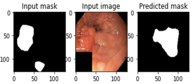
Figure 4. The input and masked images obtained for gastrointestinal images and predicting the masked regions
3.4 Base U-Net architecture
The U-Net network is divided into two parts: The first choice has a typical CNN design and is known as the contracting path. A ReLU activation unit, a layer for max-pooling, and two successive 33 convolutions make up each segment of the contracting circuit. There have been a number of changes made to this configuration. The novel features of the U-Net design may be seen in the following step of the expansion route, where each phase employs 22 up-convolutions to improve the resolution of the feature map.
The upsampled feature map is then properly trimmed and connected to the feature map of the corresponding layer within the contracting pathway. ReLU activation is followed by two more convolutions of 33. A set of 11 finishing convolutions is used to reduce the feature map to the necessary channel count and create the segmented image. In order to remove pixel attributes in the peripheries, which carry little contextual information, cropping is required. As a result, a network structure in the shape of an u appears. An important aspect of the network's contextual information distribution is that it enables the network to distinguish between objects that overlap in several regions, improving its capacity to identify things in various places.
The network's energy function is given by:
$E=\sum u(y) \log \left(q_{l(y)}(y)\right)$ (5)
where, pl is the final feature map's pixel-wise SoftMax function, which is defined as:
$q_l=\exp \left(a_l(y)\right) / \sum_{l^{\prime}=1}^l \exp \left(a_l(y)^{\prime}\right)$ (6)
and al stands for channel k activation.
3.4.1 Proposed bottle neck feature supervised U-Net
The Bottleneck U-net architecture is a variation on the well-known U-Net architecture, which is used for image segmentation tasks [23]. It combines the contracting and expanding channels of the U-Net architecture with a bottleneck layer in the middle, hence the name "Bottleneck U-Net." This change is intended to improve the model's representation power and efficiency in capturing both low-level and high-level elements in the input data.
Figure 5. Architecture of proposed bottle neck feature supervised U-Net
Figure 5 depicts the BS U-Net composition, consisting of an encoding U-Net (auto-encoder) and a segmentation U-Net (predictor). A bottleneck layer is introduced between the encoder and decoder paths in the Bottleneck U-net design. This layer is intended to extract very abstract and complicated features from incoming data, thereby functioning as a link between the contracting and expanding routes. The bottleneck layer acts as a compact representation of the critical elements of the input image, assisting in improving the model's overall segmentation performance.
Within this study, both conventional U-Nets with skip connections and those without are employed as models for constructing segmenting and encoding U-Net structures. Notably, the BS U-Net harbors substantial potential for advancement, as any U-shaped neural network has the capability to serve as a building block for constructing a U-Net framework.
To train the BS U-Net, the process begins by training the encoding U-Network using label maps as both input and labels. The encoding U-Net functions as an auto-encoder, compressing the data into a low-dimensional representation at the bottleneck layer. These encodings serve an additional supervisory role during the training of the segmentation U-Network. The training employs a comprehensive loss function for the segmentation U-Net, which combines two distinct loss functions associated with the input image and its corresponding label.
There are two primary loss components:
Euclidean loss, computed between the bottleneck feature vectors produced by the segmentation U-Net using an input image and the encoding U-Network utilizing the label.
Dice loss, which measures the dissimilarity between the network's output and the label mappings.
Given that the encoding U-Net functions as an auto-encoder, the segmentation U-Net acts as a predictor. The overall loss function used for training is a weighted average of the Euclidean loss and the Dice loss. Notably, the architecture of the BS U-Net shares similarities with the "T-L network" [24].
Monitoring the bottleneck feature vector is critical for the reasons listed below. When given the same set of intensity photos, matching label mappings, completely trained segmentation and encoding U-Nets, and pairs of intensity photographs, both instances must yield identical binary segmentation maps. As a result, any changes to the bottleneck feature vector prior to decoding are not recommended. Based on the previously supplied information, the details of the bottleneck feature vector may now be examined. Incorporating encoding information, such as supervision, has the potential to enhance segmentation performance and shorten training time, as shown by the results from the studies described in section 4.
3.5 Loss function
During the network training phase, the discrepancies between the expected and actual values were calculated using the loss functions weighted dice loss and binary cross entropy. Eqs. (2) and (3) give the formulas for computing binary cross-entropy and weighted dice loss, respectively.
$L=-W\left(\frac{2 T P}{2 T P+F P+F N}\right)$ (7)
The definitions of true positive, false positive, false negative, and false negative are denoted by the acronyms TP, FN, FP, and FN, respectively. The letter W stands for a weighting factor that is used to balance the difference in class frequency between the foreground and background.
$\begin{gathered}B=\frac{-1}{M} \sum_{i=1}^M y_i \cdot \log \log \left(q\left(y_i\right)\right)+(1-\left.y_i\right) \cdot \log \log \left(1-q\left(y_i\right)\right)\end{gathered}$ (8)
The suggested method assesses the categorization outcomes using metrics for accuracy, precision, F-score, and recall. Because of the class imbalance in the MRI dataset, these evaluations point to the necessity for model generalization. These metrics assess the overall effectiveness of the model as well as the level of inequality in class distribution. On a computer with an Intel Core i7 processor, 48 GB of RAM, and a 2 GHz CPU, the simulations are run. Cross-validation is a part of the process, and metrics for accuracy, precision, and recall that are obtained from the confusion matrix are presented.
4.1 Performance metrics
The performance measures used to evaluate the proposed method is explained as follows:
Accuracy:
The percentage of accurate predictions relative to all other predictions is what is meant by the term "accuracy." Eq. (9), when used, establishes the performance metric for accuracy.
$\operatorname{Accuracy}(\%)=\frac{\text { Number of correct predictions }}{\text { overall predictions }} \times 100$ (9)
Sensitivity:
The term sensitivity is defined as the calculation for measuring the positive ratios that are determined correctly. The sensitivity term is defined as shown in Eq. (10):
Sensitivity $(\%)=\frac{T P}{T P+F N} \times 100$ (10)
Specificity:
The term specificity is defined as the ratio of negatives which are determined correctly defined using the Eq. (11):
Specificity $(\%)=\frac{T N}{T N+F P} \times 100$ (11)
Precision:
Precision is defined as the ratio of overall positive results to overall positive predictions. Eq. (12) expresses the accuracy metric.
$\operatorname{Precision}(\%)=\frac{T P}{T P+F P} \times 100$ (12)
F-score:
The term F-score computes the accuracy for the model which is the combination of recall and precision. The F-score is measured as shown in Eq. (13):
$F-\operatorname{score}(\%)=\frac{T P}{T P+1 / 2(F P+F N)} \times 100$ (13)
The notations TP, TN, FN, and FP represent the values for "True Positive," "True Negative," "False Negative," and "False Positive" in accordance with the equations presented.
4.2 Quantitative analysis
Table 1. Results obtained for the proposed model
|
Performance Measures |
Number of Training Data |
Percentage (%) |
|
Accuracy |
2500 |
94.36 |
|
5000 |
96.21 |
|
|
7500 |
98.64 |
|
|
Sensitivity |
2500 |
87.54 |
|
5000 |
89.13 |
|
|
7500 |
93.28 |
|
|
Specificity |
2500 |
99.45 |
|
5000 |
99.62 |
|
|
7500 |
99.71 |
|
|
F-measure |
2500 |
87.25 |
|
5000 |
91.63 |
|
|
7500 |
98.12 |
|
|
Precision |
2500 |
91.05 |
|
5000 |
92.41 |
|
|
7500 |
98.08 |
Table 1 shows the performance obtained for the BS-U-Net architecture for the cross validated test data. An auto encoder creates a low dimensional encoding method for the bottleneck layer using the U-Net based functions as input. After that, the features are encoded to execute supervision for segmentation using the U-Net. The input photos are segmented, and the label corresponding to it creates an error loss function. Once the transition is performed the test dataset which submits for the evaluation of the competition organizer. Figures 6 and 7 show the results for supervising Bottleneck feature vectors condensed dimensional lowered data are represented as label maps. This transmission of data helps to control the FP and FN mistakes are reduced which in turn reduced the shape distortions. The table is evaluated and makes sense for the three perspective functions. First, the model evaluates the suggested approach by accounting for the volume of data, and an average numerical improvement of 4% is realized. Because a greater number of training samples leads to improved test performance, variation in the number of training samples is used in the evaluation process. The proposed approach is then compared to deep learning architectures.
Figure 6. The Graphical representation for the obtained error values with respect to Epochs
Figure 7. The Graphical representation for the error values obtained with respect to Epochs
5.1 Comparative analysis
The efficiency of the suggested method is assessed by comparison with current methods that displayed the result for various approaches that correspond to the KVASIR dataset that has been assessed using more traditional methods. Table 2, which offers more results than other cutting-edge techniques in the classification procedure, is what we looked at. Due to instances of misclassification, the model's accuracy was reduced because it was trained on a small sample of photos from the KVASIR dataset. The developed model lacked in the enhancement of images during the pre-processing phase and thus the datasets with labelled data showed problems for the medical image dataset. The developed LSTM-ANN model utilized a small size of data for evaluation of results which showed better memorization of the image based on their previous states. However, when the large size of data is not utilized for evaluation the LSTM-ANN model which was not able to memorize the image data. The accuracy performance failed to choose an appropriate number of parameters using GA for obtaining mutation rate and cross over. The model showed improvement in the performances that was lowered when the increase in a number of classes. Whereas the proposed model considered image samples of 7500 that utilized the proposed BS- U-Net for the process of automatically segmenting, features selection and classification that improved the learning rate as well as the performances for obtaining better precision, f-measure, and accuracy values Table 2 displays a comparison of the proposed and current models.
Table 2. Comparative analysis
|
Authors |
Dataset |
Accuracy (%) |
Precision (%) |
Measure (%) |
|
Mohapatra et al. [16] |
KVASIR |
97.25 |
97.56 |
97.59 |
|
Öztürk and Özkaya [17] |
97.90 |
94.46 |
92.64 |
|
|
Majid et al. [18] |
96.5 |
95.22 |
95.21 |
|
|
Proposed BS U-Net |
98.64 |
98.08 |
98.12 |
5.2 Implication and significance of the proposed work
The gastrointestinal tract can now more accurately detect and segment these tumours because to the implementation of a U-Net architecture with a bottleneck feature extraction component. The bottleneck feature improves the model's capacity to distinguish between healthy digestive system and tumour regions accurately by capturing crucial data and abstract representations of the tumour regions. Radiologists and physicians are relieved of some of their work by segmentation and detection of digestive system. This technique saves important time and resources while improving the effectiveness of diagnostic and treatment planning by delivering quick and reliable results. For successful treatment and better patient outcomes, gastrointestinal tract must be accurately and quickly detected. This method aids in the early detection of tumours, allowing medical personnel to intervene sooner in the course of the disease. The suggested approach advances the field of computer-aided diagnosis, deep learning, and continuing research in medical picture analysis. It lays the groundwork for more investigation and development of comparable architectural designs for other medical imaging activities.
5.3 Confounding factors
Patients with various characteristics, such as age, gender, general health, and other underlying medical issues, may be included in the study. These variables may affect how gastrointestinal tract tumours appear dataset, which could have an impact on the effectiveness and generalizability of the model. The appearance of tumours can be impacted by the presence of prior treatments or changes in tumour size brought on by progression. The model's predictions may be less accurate if these factors are not adequately taken into account. Due to variations in genetic characteristics, lifestyle choices, and illness frequency, the model's performance may change among various ethnicities and demographic groups.
The proposed BS U-Net technique was used in the current study to identify the GI anomalies. The results of the suggested approach showed that 8000 images from the KVASIR V2 dataset were used for both training and testing. The present research work utilized a raw dataset that consisted of an unbalanced size dataset for performing the process of scaling and enhancement. The proposed Bottlenecks in U-Networks are a way that forces the model for performing the input data compression and it is quite important to learn the input data compression. This compressed view of data consists of useful information which is utilized for input image reconstruction and is called as segmentation process. As a result, eight separate classifications—Z-line, pylorus, cecum, esophagitis, polyps, ulcerative colitis, dyed and lifted polyps, and dyed resection margins—are automatically applied to the precise segments. However, the handheld values were believed that gastric cancer was helpful to determine the biopsy samples taken from the patient to determine area required a useful model. The proposed methodology successfully and quickly identified cancer, reducing the amount of time needed for diagnosis. The proposed model outperformed the LSTM-ANN and GA Algorithms, with accuracy and specificity of 98.64% and 99.71, respectively. By extending the current method to handle three-dimensional images, gastrointestinal tract can be accurately segmented in three dimensions (3D). This might offer a more thorough image of tumour location and morphology, improving clinical applications.
[1] Eklöf, V., Löfgren‐Burström, A., Zingmark, C., Edin, S., Larsson, P., Karling, P., Alexeyev, O., Rutegård, J., Wikberg, M.L., Palmqvist, R. (2017). Cancer‐associated fecal microbial markers in colorectal cancer detection. International Journal of Cancer, 141(12): 2528-2536. https://doi.org/10.1002/ijc.31011
[2] Pogorelov, K., Randel, K.R., Griwodz, C., Eskeland, S.L., de Lange, T., Johansen, D., Spampinato, C., Dang-Nguyen, D.T., Lux, M., Schmidt, P.T., Riegler, M., Halvorsen, P., Kvasir. (2017). A multi-class image dataset for computer aided gastrointestinal disease detection. In Proceedings of the 8th ACM on Multimedia Systems Conference, ACM, New York, NY, USA, pp. 164-169. https://doi.org/10.1145/3083187.3083212
[3] Das, A., Acharya, U.R., Panda, S.S., Sabut, S. (2019). Deep learning-based liver cancer detection using watershed transform and Gaussian mixture model techniques. Cognitive Systems Research, 54: 165-175. https://doi.org/10.1016/j.cogsys.2018.12.009
[4] Wang, G.H., Zhao, C.M., Huang, Y., Wang, W., Zhang, S., Wang, X. (2018). Expression patterns and prognostic significance in digestive system cancers. Human Pathology, 71: 135-144. https://doi.org/10.1016/j.humpath.2017.10.032
[5] Hirsch, D., Gaiser, T., Merx, K., Weingaertner, S., Forster, M., Hendricks, A., Woenckhaus, M., Schubert, T., Hofheinz, R.D., Gencer, D. (2021). Clinical responses to PD-1 inhibition and their molecular characterization in six patients with mismatch repair-deficient metastatic cancer of the digestive system. Journal of Cancer Research and Clinical Oncology, 147(1): 263-273. https://doi.org/10.1007/s00432-020-03335-2
[6] Chen, X., Pan, Y., Liu, H., Bai, X., Wang, N., Zhang, B. (2016). Label-free detection of liver cancer cells by aptamer-based microcantilever biosensor. Biosensors & Bioelectronics, 79: 353-358. https://doi.org/10.1016/j.bios.2015.12.060
[7] Hirasawa, T., Aoyama, K., Tanimoto, T., Ishihara, S., Shichijo, S., Ozawa, T., Ohnishi, T., Fujishiro, M., Matsuo, K., Fujisaki, J., Tada, T. (2018). Application of artificial intelligence using a convolutional neural network for detecting gastric cancer in endoscopic images. Gastric Cancer, 21(4): 653-660. https://doi.org/10.1007/s10120-018-0793-2
[8] Ishioka, M., Hirasawa, T., Tada, T. (2019). Detecting gastric cancer from video images using convolutional neural networks. Digestive Endoscopy, 31(2): e34-e35. https://doi.org/10.1111/den.13306
[9] Yasuda, Y., Tokunaga, K., Koga, T., Sakamoto, C., Goldberg, I.G., Saitoh, N., Nakao, M. (2020). Computational analysis of morphological and molecular features in gastric cancer tissues. Cancer Medicine, 9(6): 2223-2234. https://doi.org/10.1002/cam4.2885
[10] Yoon, H.J., Kim, S., Kim, J.H., Keum, J.S., Oh, S.I., Jo, J., Chun, J., Youn, Y.H., Park, H., Kwon, I.G., Choi, S.H. (2019). A lesion-based convolutional neural network improves endoscopic detection and depth prediction of early gastric cancer. Journal of Clinical Medicine, 8(9): 1310. https://doi.org/10.3390/jcm8091310
[11] Raju, M.S.N., Rao, B.S. (2022). Classification of colon and lung cancer through analysis of histopathology images using deep learning models. Ingénierie des Systèmes d'Information, 27(6): 967-971. https://doi.org/10.18280/isi.270613
[12] Devi, A.G., Rao, B.S.P., Haritha, T., Mandava, V.S.R., Balaji, T., Sagar, K.V., Rao, K.K. (2023). An improved CHI2 feature selection based a two-stage prediction of comorbid cancer patient survivability. Revue d'Intelligence Artificielle, 37(1): 83-92. https://doi.org/10.18280/ria.370111
[13] Vente, C., Vos, P., Hosseinzadeh, M., Pluim, J., Veta, M. (2021). Deep learning regression for prostate cancer detection and grading in bi-parametric MRI. IEEE Transactions on Biomedical Engineering, 68(2): 374-383. https://doi.org/10.1109/tbme.2020.2993528
[14] Lee, J.H., Kim, Y.J., Kim, Y.W., Park, S., Choi, Y., Kim, Y.J., Park, D.K., Kim, K.G., Chung, J.W. (2019). Spotting malignancies from gastric endoscopic images using deep learning. Surgical Endoscopy, 33(11): 3790-3797. https://doi.org/10.1007/s00464-019-06677-2
[15] Horiuchi, Y., Aoyama, K., Tokai, Y., Hirasawa, T., Yoshimizu, S., Ishiyama, A., Yoshio, T., Tsuchida, T., Fujisaki, J., Tada, T. (2020). Convolutional neural network for differentiating gastric cancer from gastritis using magnified endoscopy with narrow band imaging. Digestive Diseases and Sciences, 65(5): 1355-1363. https://doi.org/10.1007/s10620-019-05862-6
[16] Mohapatra, S., Nayak, J., Mishra, M., Pati, G.K., Naik, B., Swarnkar, T. (2021). Wavelet transform and deep convolutional neural network-based smart healthcare system for gastrointestinal disease detection. Interdisciplinary Sciences: Computational Life Sciences, 13(2): 212-228. https://doi.org/10.1007/s12539-021-00417-8
[17] Öztürk, Ş., Özkaya, U. (2020). Gastrointestinal tract classification using improved LSTM based CNN. Multimedia Tools and Applications, 79(39-40): 28825-28840. https://doi.org/10.1007/s11042-020-09468-3
[18] Majid, A., Khan, M.A., Yasmin, M., Rehman, A., Yousafzai, A., Tariq, U. (2020). Classification of stomach infections: A paradigm of convolutional neural network along with classical features fusion and selection. Microscopy Research and Technique, 83(5): 562-576. https://doi.org/10.1002/jemt.23447
[19] Liu, S., Liu, S., Ji, C., Zheng, H., Pan, X., Zhang, Y., Guan, W., Chen, L., Guan, Y., Li, W., He, J., Ge, Y., Zhou, Z. (2017). Application of CT texture analysis in predicting histopathological characteristics of gastric cancers. European Radiology, 27(12): 4951-4959. https://doi.org/10.1007/s00330-017-4881-1
[20] Sundaram, P.S., Santhiyakumari, N. (2019). An enhancement of computer aided approach for colon cancer detection in WCE images using ROI based color histogram and SVM2. Journal of Medical Systems, 43(2): 29. https://doi.org/10.1007/s10916-018-1153-9
[21] Wang, Y., Peng, T., Duan, J., Zhu, C., Liu, J., Ye, J., Jin, M. (2020). Pathological image classification based on hard example guided CNN. IEEE Access, 8: 114249-114258. https://doi.org/10.1109/ACCESS.2020.3003070
[22] Kvasir Dataset. https://www.kaggle.com/datasets/meetnagadia/kvasir-dataset.
[23] Girdhar, R., Fouhey, D.F., Rodriguez, M., Gupta, A. (2016). Learning a predictable and generative vector representation for objects. In European Conference on Computer Vision, Springer, pp. 484-499. https://doi.org/10.48550/arXiv.1603.08637
[24] Oktay, O., Ferrante, E., Kamnitsas, K., Heinrich, M., Bai, W., Caballero, J., Cook, S.A., de Marvao, A., Dawes, T., O‘Regan, D.P., Kainz, B., Glocker, B., Rueckert, D. (2017). Anatomically constrained neural networks (ACNNs): Application to cardiac image enhancement and segmentation. IEEE Transactions on Medical Imaging, 37(2): 384-395. https://doi.org/10.1109/tmi.2017.2743464