Yuzhong Liu![]() | Tianfan Zhang*
| Tianfan Zhang*![]() | Zhe Li
| Zhe Li![]() | Lequan Deng
| Lequan Deng![]()
© 2023 IIETA. This article is published by IIETA and is licensed under the CC BY 4.0 license (http://creativecommons.org/licenses/by/4.0/).
OPEN ACCESS
Motion perception, pivotal to myriad specialized tasks, necessitates the enhancement of proficiency through sustained repetition of perception-action cycles to meet standard benchmarks. Attaining advanced skill levels often demands additional practice. However, traditional pedagogical and evaluation systems predominantly hinge on the subjective experiences of instructors and evaluators. This dependence precipitates two principal challenges in the domain of motion perception-related professional work. Firstly, learners grapple with securing timely, adequate guidance during learning and practice, given the slow, trial-and-error nature of key point acquisition. Secondly, objective evaluation, fraught with instability, fails to consistently deliver accurate quantitative assessments, thereby adversely impacting the learning process. In response to these challenges, this study introduces a deep learning-based approach for standardized evaluation and human pose estimation. The methodology begins with the utilization of OpenPose for body joint detection. This is followed by a Deep Neural Network (DNN)-informed strategy for posture information extraction. Lastly, leveraging our team's extensive experience in dance instruction, a novel method for describing and discerning differences in dance movements is proposed. This approach enables a quantitative evaluation and provides intuitive feedback on the mechanics of dance movements, thereby enhancing the monitoring of participants' progress. Validated experimentally, the proposed methodology demonstrates precision in motion perception and quantitative evaluation. It not only offers practical guidance for enhancing the quality of dance instruction but also provides a valuable reference for other applications.
dance training, OpenPose, human pose estimation (HPE), pose feature description, pose matching
Traditional dance teaching emphasizes on the consistency of dancing movement, ignoring the students’ individual characteristics. Whereas, personalized and diversified dance education is oriented to different objects and goals according to students’ individual conditions, educational backgrounds, and developmental needs. The traditional dance teaching model cannot effectively achieve the goal of cultivating diversified dance talents [1]. In particular, the training of dance movement, as one of the fundamental parts in dance teaching, covers a wide range of standard movements such as jumping jack, flick Jump, leg curl jump, and knee lift jump etc. But in the dance training, some incorrect poses may influence the training quality, the students’ dance scores, and even lead to delayed graduation etc. [2]. Therefore, it is necessary to identify the human pose in the training process and timely solve the problems existing in dance training in colleges, thus improving the effect of dancing training. Currently the research on the real-time identification of human pose has received wide attention from all walks of life. Especially, following the development of big data and image information processing technology, a real-time human pose estimation method for dance training has been developed to more effectively correct the human pose in college dance training, and improve the training effect. In view of the above, the study on the relevant HPE for college dance training is of great significance for optimizing the teaching quality of dance training [3]. This paper aims to explore a highly robust, high-precision method for correcting the human poses through the study on the standard pose movement of dances.
In summary, it urgently needs to solve the problem of how to express the subjective experience of professional evaluators quantitatively and reproduce it intuitively in the dance teaching and evaluation. To solve the problems above, this paper investigates a deep learning-based HPE and evaluation method. First, OpenPose is applied to achieve the recognition of human skeleton and key points, and to express the body language of the test subjects quantitatively; then, a DNN-based pose estimation method is established to obtain the information of human pose and the main characteristics of the actions being completed by the test subjects, while considering the individual differences the quantitative expression library of standard dance movements is built by collecting standard dance movements of different professional dance teachers; the evaluation robustness is obtained by learning the allowable feature differences; finally, the feature description of dance movement and the method of determining the differences were developed to realize its quantitative evaluation and intuitive feedback mechanism, thereby better monitoring the students’ learning.
Human Pose Estimation (HPE) is usually performed based on the skeleton. Skeleton-Based Action Recognition (SAR) has been a hot research topic in the field of computer vision. However, we are still faced with challenges such as occlusion, insufficient training data and depth ambiguity. 2D HPE of images and videos with 2D pose annotations can be easily implemented, while the HPE of a single person based on deep learning has reached the optimal.
Using AlexNet [5] as a backbone, Toshev and Szegedy [4] proposed a cascaded deep neural network regressor called DeepPose to learn key points from images. Due to the excellent performance of DeepPose, the research paradigm of HPE started to shift from classical methods to deep learning, especially Convolutional Neural Networks (CNN) [6]. Based on GoogLeNet [7], Carreira et al. [8] proposed an Iterative Error Feedback (IEF) network. IEF is a self-correcting model that injects the prediction error into the input space, and gradually changes the initial solution. Sun et al. [9], introduced a structure-aware regression method based on ResNet-50 [10], called "component pose regression", which replaces the traditional joint-based representation with a skeleton-based reparameterized representation that incorporates body information and pose structure. Luvizon et al. [11] gave an end-to-end regression method for HPE, transforming the feature map into joint coordinates in a fully differentiable framework using a softargmax function.
Li et al. [12], based on the encoder-decoder architecture of transformers, designed a cascaded transformer-based model, PRTR, which can acquire spatial relationships from joints and perform key point prediction by regression inference [13]. Good properties for encoding rich pose information are crucial for regression-based approaches. Multitask learning is a popular strategy for learning better feature representations [14]. By sharing and representation among related tasks, the model can better generalize the pose estimation task. For this, Li et al. [15] proposed a heterogeneous multitasking framework consisting of two tasks: predicting the joint coordinates from a complete image by regressors and detecting body parts from image patches using sliding windows. Fan et al. [16] developed a two-source CNN for joint detection and joint localization to determine whether body joints are included in the patch as well as their exact location. Each task corresponds to a loss function, and the combination of two tasks will lead to improved results. Luvizon et al. [17] learned a multitasking network to jointly process 2D/3D pose estimation and action recognition from video.
The dance game "Just Dance" [18] developed by Ubisoft Entertainment are among the most popular types of exergames. It has a rich library of dances and an advanced scoring mechanism, so as to be introduced in the dance teaching. However, the limited development environment and evaluation algorithm hinder its further development in the academic research field.
In summary, DeepPose has a novel architecture with high accuracy for pose estimation of real-world images. It achieves 2D pose estimation of the human body from videos and images with more accurate localization of key points [19]. STGCN [20] can help to realize autonomous learning of the data’s spatial and temporal characteristics. DPRL [21] selects the more important ones among all frames for recognition, thus improving the detection speed of key points.
Usually, there are two ways to obtain skeleton points: one is to obtain point cloud data through special devices such as depth sensors [22], and then perform pose recognition through the point cloud, to obtain the skeleton and key points, which can ensure high recognition accuracy, but relying on special equipment with a huge amount of computation, and has a depth-of-field limitation, being unfavorable to the environment of multiple dancing [23]; the other one is realized by ordinary camera such as OpenPose pose recognition algorithm, which can obtain high accuracy under various working conditions with no need of special equipment, and also gradually becomes the mainstream scheme of pose recognition.
3.1 Skeleton and key point extraction
To ensure the accuracy, this paper selects OpenPose [19] as the base recognition method for skeleton and key point extraction. OpenPose proposes the first bottom-up association score representation through Part Affinity Fields (PAFs) [24], which is a set of two-dimensional vector fields encoding the position and orientation of the limbs on the image domain. The system takes the color image in $\omega \times h$ as input and generates the two-dimensional anatomical key point locations of each person in the image as output. First, the feedforward network predicts both a set of 2D confidence maps $S$ of body part locations and a set of 2D vector fields $L$ of part affinities that encode the degree of association between parts. The set $S=$ $\left(S_1, S_2, \cdots, S_J\right)$ has a confidence map, one for each part, where $S_j \in \mathbb{R}^{\omega \times h}$. The set $L=\left(L_1, L_2, \cdots, L_C\right)$ has a vector field, one for each limb (limb), where $L_C \in \mathbb{R}^{\omega \times h \times 2}, c \in\{1, \cdots, C\}$. Finally, the confidence maps and affinity fields are parsed by greedy inference to output the two-dimensional key points of all people in the image.
3.2 Pose representation
In the pose representation, the positions of all body joints $k$ are encoded into a pose vector $y$, to be defined as $y=$ $\left(y_1^T, y_2^T, \ldots, y_i^T, \ldots, y_k^T\right)^T, i \in\{1, \ldots, k\}$, where $y_i$ contains the $x$ and $y$ coordinates of the $i^{t h}$ joint. The labeled image is denoted by $(x, y)$ where $x$ represents the image data and $y$ is the ground truth pose vector.
Since the joints of the human body are represented by the absolute coordinates in the image, it is beneficial to perform normalization in the $b$ containing the human body ROI. Generally, the ROI's $b$ can represent the complete image containing the human body, such that $b$ is defined by the center $b_c \in \mathbb{R}^2$, width $b_w$, and height $b_h: b=\left(b_c, b_w, b_h\right)$. The joints $y_i$ can then be translated by the box center and scaled by the box size, which is called normalization by $b$.
$N\left(y_i ; b\right)=\left(\begin{array}{cc}1 / b_\omega & 0 \\ 0 & 1 / b_h\end{array}\right)\left(y_i-b_c\right)$ (1)
Furthermore, the same normalization can be applied to the pose vector $N(y ; b)=\left(\ldots, N\left(y_i ; b\right)^T, \ldots\right)^T$ for a normalized pose vector. Afterwards, the cropping of the image is represented by the bounding box B using $N(x ; b)$, which is actually the image normalization by the box.
3.3 DNN regression-based pose estimation
In this study, the pose estimation problem is considered as a regression. By using the function $\psi(x ; \theta) \in \mathbb{R}^{2 k}$, the image $x$ is regressed to a normalized pose vector, where $\theta$ is the model parameter. Thus, based on the normalized transformation from Eq. (1), the pose prediction $y^*$ is read in absolute image coordinates as:
$\mathrm{y}^*=N^{-1}(\psi(N(x)) ; \theta)$ (2)
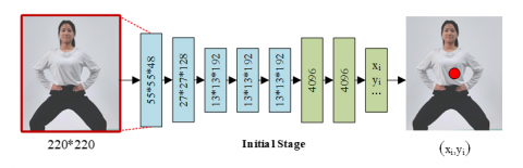
where, $\psi$ denotes the property and complexity of the method. Such a convolutional network consists of several layers - each layer is a linear transform, followed by a nonlinear transform. Considering that DNN architectures excel in classification and localization problems, the architecture of $\psi$ is built according to the Ref. [5], as shown in Figure 1. The entire network consists of seven layers.
Figure 1. Schematic diagram of DNN-based pose regression framework
C denotes the convolutional layer, LRN (Local Response Normalization) is the local response normalization layer [25], $\mathrm{P}$ is the pooling layer, and $\mathrm{F}$ is the fully connected layer. Only the $\mathrm{C}$ and $\mathrm{F}$ layers contain learnable parameters, while the rest are parameter less. Both $\mathrm{C}$ and $\mathrm{F}$ layers consist of a linear transformation and a nonlinear transformation (using rectified linear units (PRelu)). For the C layers, the size is defined as width $\times$ height $\times$ depth, where the first two dimensions are spatially meaningful, while the depth defines the number of filters. The filter sizes are $11 \times 11$ and $5 \times 5$ for the first two layers and $3 \times 3$ for the remaining three. The pooling, when applied to all three layers, helps to improve performance despite the reduced resolution. The input to the network is a $220 \times 220$ image and stride $=4$.
In the training, the difference with the Ref. [5] can be defined as the loss (loss). To avoid the classification loss, the linear regression is trained on the last network layer to predict the pose vector by minimizing the distance $L_2$ between the predicted and the true pose vector. When the true pose vector is defined in absolute image coordinates and the pose size varies from image to image, the training set $D$ is normalized using the normalization method in Eq. (1) as follows:
$D_N=\{(N(x), N(y)) \mid(x, y) \in D\}$ (3)
Then the L2 loss of the optimal network parameters is given as:
$\arg \min _\theta \sum_{(x, y) \in D_N} \sum_{i=1}^k\left\|y_i-\psi_i(x ; \theta)\right\|_2^2$ (4)
where, the parameter $\theta$ is optimized for the use of backpropagation in a distributed online process. The training parameters are set to be mini-batch $=128$, and adaptive gradient is updated and calculated with reference to the study [26]; learning rate $=0.0005$. due to the large number of parameters in the model and the relatively small size of the dataset, the images are enhanced by lots of random transformations (rotation, mirroring, etc.) in the training.
3.4 Cascaded pose regression
DNN regression-based pose estimation is made for the complete image, so it is context dependent. However, due to its fixed input size of 220×220, the network has limited ability to view details - it learns filters that capture the coarse pose attributes. Despite its fast and coarse estimate of pose, it is not accurate enough to eventually localize each key joint of the body. Also, this can be done by changing the size of the input image, but leading to a significant computational complexity. Therefore, it is a good solution to improve the accuracy by training a cascaded pose regressor.
First, the initial pose is estimated, and then additional DNN regressors are trained to predict joint position changes and displacement. In this way, each subsequent stage can be considered as a refinement of the current predicted pose, as shown in Figure 2:
Figure 2. Framework of cascaded pose regressors based on DNN
Thus, only the predicted subgraph of the joint position is cropped each time, and then the key regression function is applied to that subgraph. In this way, even if the size of the input image cannot be changed, we still obtain the detailed features on a finer scale, and then improve the accuracy because the subgraph contains only the joint image as much as possible.
Besides, the same network architecture is used for all stages of cascade, so it only needs to learn different network parameters. The stage $s \in\{1, \ldots, S\}$ denotes the network parameters of the total $\mathrm{S}$ cascade stage, and $\theta_s$ is the learned network parameters. Then, the positional displacement regression function reads $\psi\left(x ; \theta_s\right)$. To specify a given joint position $y_i$, we consider a joint box $b_i$ that captures the surrounding sub-images of $y_i: y_i: b_i(y ; \sigma)=$ $\left(y_i, \sigma \operatorname{diam}(y), \sigma \operatorname{diam}(y)\right)$ with the $i$-th joint as the center and $\theta$ as the scale of the pose diameter. The pose diameter $(y)$ is defined as the distance between relative joints on the human torso, such as the left shoulder and the right hip, depending on the specific posture definition and data set.
Thus, at stage $s=1$, starting from an enclosing box $b^0$, it either contains the complete image or is obtained by the human detector. Thus, an initial pose Stage 1 is obtained:
$\begin{align} & Stage\ 1:{{y}^{1}}\leftarrow {{N}^{-1}}(\psi (N(x;{{b}^{0}});{{\theta }_{1}});{{b}^{0}}) \\ & \quad \cdots \\ & Stage\ S:y_{i}^{s}\leftarrow y_{i}^{s-1}+{{N}^{-1}}(\psi (N(x;b);{{\theta }_{s}});b) \\ & \quad \quad \quad \quad \quad \quad for\quad b=b_{i}^{(s-1)} \\ & \quad \quad \quad \quad \quad b_{i}^{s}\leftarrow (y_{i}^{s},\sigma diam({{y}^{s}}),\sigma diam({{y}^{s}})) \\ \end{align}$ (5)
In each subsequent stage $s \geq 2$, for all joints $i \in\{1, \ldots k\}$ a regression function is applied to the sub-images defined in the previous stage $y_i^s-y_i^{(s-1)}$. First, a regression is applied towards the refined displacement $b_i^{(s-1)}$. Then, the new joint box $b_i^s$ is estimated. The network parameters $\theta_1$ are trained according to the Eq. (4). In the next stages ( $s \geq 2$ ), the training is performed in the same way, with only one big difference. In the training example $(x, y)$, each joint $i$ uses a different enclosing box ${{y}_{i}}^{(s-1)},\sigma \text{diam}(y),\sigma \text{diam}(y)$ centered on the prediction of the same joint obtained in the previous stage and normalized so as to adjust the training in the current stage according to the model of the previous stage.
Next, the training data is then augmented by using multiple normalizations for each image and joint. Instead of using only the predictions from the previous stage, we generate simulated predictions. This can be achieved by randomly replacing the true positions of the joint $i$ with vectors sampled randomly from a two-dimensional normal distribution $N_i^{(s-1)}$, with means and variances equal to those of the displacements $\left(y_i^{(s-1)}-y_i\right)$ observed in all examples of the training data. The complete augmented training data can be defined by: firstly, sample an example and a joint uniformly from the original data, and then generate simulated predictions based on the displacement $\theta$ sampled from $N_i^{(s-1)}$.
$\begin{aligned} D_A^s= & \left\{\left(N(x ; b), N\left(y_i ; b\right)\right) \mid\left(x, y_i\right) \sim D, \delta \sim \mathrm{N}_i^{(s-1)},\right. \\ & \left.b=\left(y_i+\delta, \sigma \operatorname{diam}(y)\right)\right\}\end{aligned}$ (6)
The training objective of the cascade stage S is shown in Eq. (4), with special attention to using the correct normalization for each joint.
$\theta_{\mathrm{s}}=\arg \min _\theta \sum_{(x, y) \in D_A^s}\left\|y_i-\psi_i(x ; \theta)\right\|_2^2$ (7)
3.5 Feature description and determination of dance movement
Three elements are usually considered when evaluating the dance movements [18]: timing, amplitude, and direction.
Timing: any movement, can be broken down into three parts: static, dynamic, and static. The dance movement of the “start and finish” must be at the right timing for a higher evaluation;
Amplitude: the amplitude of the movements should be basically consistent with the standard (here refers to the standard library), since persons vary in height.
Direction: it’s not required strictly. The right direction can make the front and back of the action linked more smoothly, thus resulting in higher evaluations.
Since errors are inevitable, we need to consider how to define the criterion of "tolerable error". This relies on a large sample of dancers' movements and supervised training by experts. In local practice, 5% variation is acceptable, or it’s difficult to distinguish, e.g., if jumping jack requires a knee angle of no less than 90 degrees, then a range of 85° or more is considered acceptable (in fact, larger deviations may be acceptable, depending on the overall postural finish at the time - potentially masking minor details).
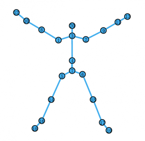
The above evaluations are highly dependent on expert experience. Combining the human movement as well as the structural characteristics of the human body, this paper chooses the 20 nodes defined by Deng et al. [22] to represent the dance movements, as shown in Figure 3.
Figure 3. The 20 nodes defined and numbered by Kinect
Twenty skeletal joint points are extracted, to constitute the first 20 feature values of the feature vector T for the joint coordinate point, and then a (quantitative) standardized description of a specific action is performed for these 20 feature values. These features can be expressed as:
$T_i=P_i\left(x_i, y_i, z_i\right), i=1,2 \ldots, 20$ (8)
where, $x_i$ represents the projection of the point $P_i$ on the $x$ coordinate axis; $y_i$ is the projection of $P_i$ on the $y$ coordinate axis; $z_i$ is the one on the $z$ coordinate axis. The lens location is the origin of the coordinates. Assuming that the adjacent standard pose feature point is set as $\left(x_n, y_n, z_n\right)$, and the imitation pose feature point is $\left(x_m, y_m, z_m\right)$, then the feature vector values corresponding to the two pose feature points are
$n=\left(x_0, y_0, z_0\right)-\left(x_1, y_1, z_1\right)$ (9)
From Eq. (6), the set of feature vectors can be derived as $P=\left\{n_0, n_1, n_2, \ldots, n_8\right\}$, which is called the pose feature descriptor to describe the human action pose, as shown in in subgraph (a) of Figure 4.
Figure 4. Pose calibration and determination
Once a standard pose model is defined, the actual pose of the current test subject can be compared with the standard. As shown in subgraph (b) of Figure 4, if exceeding the tolerance error, the test pose can be considered to be non-standard, i.e., there are two problems with the movement: first, the angle between the thigh and the calf is not 120°; then, the calf is not perpendicular to the ground, but has an inward tilt. Therefore, it’s determined that such action needs to be corrected.
3.6 Pose matching of human movement
After acquiring the feature descriptors of the human movements, the matching and recognition problem between two poses is transformed into the discrepancy of feature descriptor. Regarding this problem, it can be judged by comparing the angle values between the feature vectors corresponding to the standard pose and the mimic pose descriptors. Suppose the feature vectors of the standard pose and the imitation pose feature descriptor are set as $a\left(x_{s t}, y_{s t}, z_{s t}\right)$ and $b\left(x_{r e}, y_{r e}, z_{r e}\right)$, respectively, then the cosine value of the angle value between the two poses is:
$\cos _{a i}=\frac{x_{s t} \cdot x_{r e}+y_{s t} \cdot y_{r e}+z_{s t} \cdot z_{r e}}{\sqrt{x_{s t}{ }^2+y_{s t}{ }^2+z_{s t}^2} \cdot \sqrt{x_{r e}{ }^2+y_{r e}{ }^2+z_{r e}^2}}$ (10)
In Eq. (6), $a_i$ is the angle values in the range of $\left[0,180^{\circ}\right]$. From this, the set of angle values can be derived as $\theta=$ $\left\{a_0, a_1, a_2, \ldots, a_8\right\}$, and the difference between the two poses can be expressed in this way. As a result, the sum of the angle values is given as:
$a_{s u}=\sum_{i=0}^8 a_i$ (11)
The weight of each angle value is calculated as:
$\omega_i=\left(1-e-\frac{a_i}{a_{s u}}\right) /\left(\sum_{i=0}^8 1-e-\frac{a_i}{a_{s u}}\right)$ (12)
Based on the Eq. (12), a set of weight values can be derived as $W=\left\{\omega_0, \omega_1, \cdots, \omega_8\right\}$, so as to obtain the normalized angle values:
$D=\sum_{i=0}^8 a_i, \omega_i$ (13)
The normalized angle value parameter D derived from Eq. (13) can represent the degree of difference between the standard pose and the imitation pose. On this basis, the accuracy of matching between the two poses can be identified by introducing the D value into the formula of pose matching, which is given by:
$S= \begin{cases}f\left(a_{\text {max }}\right) \cdot\left[\left(D_{s t}-D\right) \cdot \frac{100-S_{s t}}{D_{s t}}+S_{s t}\right] & , 0 \leq D \leq D_{s t} \\ 0 & , D>D_{s t}\end{cases}$ (14)
where, S represents the recognition accuracy of pose matching, in the value range of $[0,100] ; D_{s t}$ is the threshold of the preset standard angle difference; $S_{s t}$ is the preset baseline matching parameter; $f\left(a_{\max }\right)$ is the limb offset limit function, which mainly benefits from the penalty factor of pose matching accuracy. The larger the value of $S$, the better the match between the two poses; the smaller the value $D_{s t}$, the more severe the match accuracy between the two poses. The specific calculation formula is given as:
$f\left(a_{\text {max }}\right)= \begin{cases}1-\frac{0.3}{M^2} \cdot a_{\max }^2 & , 0 \leq a_{\text {max }} \leq \sqrt{10 / 3 M} \\ -\frac{0.3}{M^2} \cdot a_{\max }^2 & , a_{\max }>\sqrt{10 / 3 M}\end{cases}$ (15)
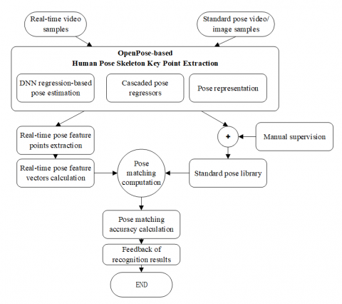
In this paper, the experiments were conducted as shown in Figure 5.
Figure 5. Experimental idea
4.1 Sample set
The public datasets of human movements mainly include:
The NTU-RGB+D [27] dataset comprises two distinct versions: the NTU RGB+D 60, containing 56,880 sample data across 60 actions, and the NTU RGB+D 120, an expanded version encompassing all previous data and an additional 60 categories, culminating in a total of 114,480 samples. Each dataset includes RGB video, depth map sequences, 3D skeletal data, and infrared (IR) video for every sample, all captured simultaneously by three Kinect V2 cameras. The RGB video resolution is set at 1920x1080, while both the depth map and IR video maintain a resolution of 512x424. The 3D skeletal data includes the 3D coordinates of 25 body joints per frame. It should be noted that the NTU RGB-60, while not specifically dedicated to dance movements, possesses a strong universality and embodies "daily" characteristics. This versatility is a significant factor in our decision to select it as the basic testing methodology.
MSR-Action3D [28] dataset has a total of 20 movements: high swing, horizontal swing, whack, catch, forward punch, high throw, draw cross, draw hook, draw circle, clap, two-handed wave, side punch, bend, front kick, side kick, jog, tennis racket swing, tennis serve, golf club swing, pick-up, and throw. 10 participants performed each movement 2 to 3 times.
The Microsoft MSRC-12 movement dataset from the Cambridge Research Institute [29], collected 12 physical movements containing gesture movements of 30 participants. The original dataset contained 719,359 frames of action data.
The UTKinect-Action dataset [30] collected 10 types of movements: walking, sitting, standing up, picking up, holding an object, throwing, pushing, pulling, waving, and clapping. Action data were collected from 10 performers, and each action was executed twice.
First, pre-training weights are obtained by learning and training of these sample sets. Then fine-tuning (fine-tuning) is performed using the dataset related to the dance.
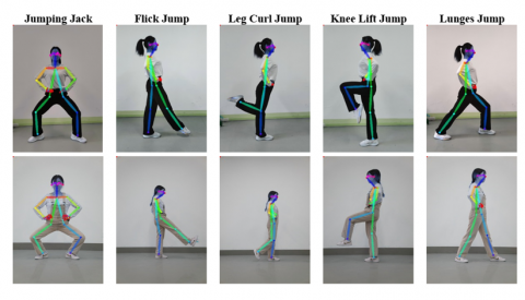
Five typical movements are selected for the dance design: jumping jack, flick Jump, leg curl jump, knee lift jump, and lunges jump, as shown in Table 1.
Table 1. Dance movement design: five typical movement examples and movement essentials
|
Jumping Jack |
Flick Jump |
Leg Curl Jump |
Knee Lift Jump |
Lunges Jump |
|
In the split-legged knee squat, separate the two toes naturally, flex the knee joint in the direction of the toes, keep the knee joint angle not less than 90 degrees, and ensure the heel to land on the ground. |
Choose one leg as the power leg, make the two knees come together, while straighten the other leg, and maintain the power leg at an angle of about 30°. |
Keep the supporting leg flexible, both knees together, make hips and knees fall in a line, and ensure the heel close to the hip. |
Lift the knee first and keep the thigh parallel to the ground, knee at 90 degrees to the body, toe against the dominant leg, foot taut. |
Make one leg back swing from the toe to the forefoot, without landing the heel, keep the toe towards the front. Leans slightly forward, stand waist and tuck the abdomen. |
The essentials of each movement vary, but all these five movements have the same requirements for upper body, i.e., the head and torso are basically vertical and the arms are crossed at the waist.
4.2 Results analysis
The SPSS statistical analysis software and MATLAB were utilized to test the efficacy of the model in achieving real-time recognition of dance poses. The frame rate of visual sampling for dance poses was established at 100 FPS, with a feature resolution of 1920x1080 RGB. The duration of visual information acquisition was set at 12 seconds, yielding a sample data length of 1200 and a training sample size of 240 frames. In conjunction with the NTU RGB D 60 dataset, the training was executed to yield statistical analysis results using different dance movements as test samples.
Table 2. Testing based on NTU RGB-D 60 dataset.
|
Action |
Average Accuracy |
Action |
Average Accuracy |
|
A5: drop |
100% |
A27: jump up |
100% |
|
A6: pick up |
100% |
A31: point to something |
100% |
|
A7: throw |
95% |
A32: taking a selfie |
96% |
|
A8: sit down |
100% |
A33: check time (from watch) |
95% |
|
A9: stand up |
100% |
A35: nod head/bow A |
100% |
|
A10: clapping |
92% |
A38: salute |
100% |
|
A20: put on a hat/cap |
100% |
A39: put palms together |
93% |
|
A21: take off a hat/cap |
94% |
A40: cross hands in front |
100% |
Prior to testing dance action instances, basic motion tests were conducted using the NTU RGB-D 60 dataset. Sixteen actions, such as A5, A6...A40, were selected due to their resemblance to dance movements. The test results are exhibited in Table 2. It is evident that the accuracy is relatively high for most actions, while for actions A7, A10, A21, A32, A33, and A39 the accuracy is comparatively low. Notably, A10 and A39, due to their significant similarity, led to misclassifications during recognition.
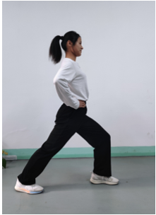
In order to test the recognition effect of each group of movements for different individuals and background environments, the test sample was increased to 10. Figure 6 shows the recognition effect of one group of movements. If the current subject's movement is the same as the standard movement (or within the tolerance range), it is considered as correct; if recognized as another movement or beyond the tolerance range, it shall be wrong.
Figure 6. Test results: standard and non-standard movements
Besides, the camera shooting distance was consciously changed in the test, in order to test the robustness of the evaluation model and to simulate the actual application environment in which the dancers would change their relative positions with the camera due to the need of dance expression. For example, a more distant view was adopted for groups 2 and 3 in Figure 6, and a closer view was for group 4 in Figure 6.
As illustrated in Table 3, the test results reveal that all groups completed the tasks competently. However, the mean statistical analysis indicates a substantial error rate (~5%) for Movement Essential 3 (Leg curl jump). This error distribution underscores the complexity of the movement and the participants' level of proficiency. Consequently, instructors can 1) modulate their teaching emphasis based on the overall statistical deviation and 2) offer personalized instruction tailored to the students' individual requirements. Additionally, students can proactively adjust their movements in accordance with the evaluation results to achieve improved scores.
Table 3. Recognition rate for five groups of movements
|
Test Subject |
Standard or Not |
Jumping Jack |
Flick Jump |
Leg Curl Jump |
Knee Lift Jump |
Lunges Jump |
|
1 |
Standard |
100% |
100% |
100% |
100% |
100% |
|
Non-standard |
100% |
100% |
100% |
100% |
100% |
|
|
2 |
Standard |
95% |
100% |
100% |
100% |
100% |
|
Non-standard |
100% |
100% |
100% |
100% |
100% |
|
|
3 |
Standard |
96% |
100% |
100% |
100% |
100% |
|
Non-standard |
95% |
100% |
100% |
100% |
92% |
|
|
4 |
Standard |
98% |
100% |
100% |
100% |
100% |
|
Non-standard |
100% |
100% |
100% |
95% |
99% |
|
|
5 |
Standard |
97% |
100% |
100% |
100% |
100% |
|
Non-standard |
100% |
100% |
98% |
100% |
99% |
|
|
6 |
Standard |
99% |
100% |
100% |
99% |
100% |
|
Non-standard |
100% |
99% |
100% |
100% |
100% |
|
|
7 |
Standard |
100% |
100% |
100% |
100% |
100% |
|
Non-standard |
100% |
100% |
100% |
95% |
100% |
|
|
8 |
Standard |
100% |
97% |
100% |
99% |
100% |
|
Non-standard |
100% |
100% |
100% |
100% |
97% |
|
|
9 |
Standard |
98% |
90% |
9% |
100% |
100% |
|
Non-standard |
86% |
100% |
99% |
99% |
100% |
|
|
10 |
Standard |
98% |
93% |
94% |
100% |
91% |
|
Non-standard |
100% |
99% |
100% |
96% |
100% |
|
|
AVG. |
/ |
98% |
99% |
95% |
99% |
99% |
In traditional teaching and evaluation, the evaluation system highly depends on the teachers and judges’ experience, resulting in slow feedbacks of the movements and a trial-error teaching process. Moreover, due to the subjective factors, it is difficult to achieve uniform and accurate quantitative evaluation. To solve this, the authors develop a deep learning-based method for human pose recognition and standardized evaluation. Firstly, it realizes the recognition of human skeleton and key points based on OpenPose; then, a DNN-based pose estimation method is established to acquire the individual’s pose information; finally, it builds an approach for describing the features and determining the differences between dance movements to realize the quantitative dance movement evaluation and intuitive feedback mechanism, thereby better monitoring the learning situation of the students.
[1] Mao, R. (2021). The design on dance teaching mode of personalized and diversified in the context of internet. E3S Web of Conferences, 251: 03059. https://doi.org/10.1051/e3sconf/202125103059
[2] Saearani, M.F.T.B., Chan, A.H., Abdullah, N.N.M.L. (2021). Pedagogical competency of dance instructors in the training of Malay court dance skills among upper secondary students at Johor national art school. Harmonia: Journal of Arts Research and Education, 21(2): 221-232. https://doi.org/10.15294/harmonia.v21i2.31668
[3] Camurri, A., El Raheb, K., Even-Zohar, O., et al. (2016). WhoLoDancE: Towards a methodology for selecting motion capture data across different dance learning practice. In Proceedings of the 3rd International Symposium on Movement and Computing, Thessaloniki, Greece, pp. 1-2. https://doi.org/10.1145/2948910.2948912
[4] Toshev, A., Szegedy, C. (2014). Deeppose: Human pose estimation via deep neural networks. In 2014 IEEE Conference on Computer Vision and Pattern Recognition, Columbus, USA, pp. 1653-1660. https://doi.org/10.1109/CVPR.2014.214
[5] Krizhevsky, A., Sutskever, I., Hinton, G.E. (2017). Imagenet classification with deep convolutional neural networks. Communications of the ACM, 60(6): 84-90. https://doi.org/10.1145/3065386
[6] Wu, Q., Wu, Y., Zhang, Y., Zhang, L. (2022). A local-global estimator based on large kernel CNN and transformer for human pose estimation and running pose measurement. IEEE Transactions on Instrumentation and Measurement, 71: 1-12. https://doi.org/10.1109/TIM.2022.3200438
[7] Szegedy, C., Liu, W., Jia, Y., et al. (2015). Going deeper with convolutions. In 2015 IEEE Conference on Computer Vision and Pattern Recognition (CVPR), Boston, USA, pp. 1-9. https://doi.org/10.1109/CVPR.2015.7298594
[8] Carreira, J., Agrawal, P., Fragkiadaki, K., Malik, J. (2016). Human pose estimation with iterative error feedback. In 2016 IEEE Conference on Computer Vision and Pattern Recognition (CVPR), Vegas, USA, pp. 4733-4742. https://doi.org/10.1109/CVPR.2016.512
[9] Sun, X., Shang, J., Liang, S., Wei, Y. (2017). Compositional human pose regression. In 2017 IEEE International Conference on Computer Vision (ICCV), Venice, Italy, pp. 2602-2611. https://doi.org/10.1109/ICCV.2017.284
[10] He, K., Zhang, X., Ren, S., Sun, J. (2016). Deep Residual Learning for Image Recognition. In 2016 IEEE Conference on Computer Vision and Pattern Recognition (CVPR), pp. 770-778. https://doi.org/10.1109/IEEESTD.2001.92771
[11] Luvizon, D.C., Tabia, H., Picard, D. (2019). Human pose regression by combining indirect part detection and contextual information. Computers & Graphics, 85: 15-22. https://doi.org/10.1016/j.cag.2019.09.002
[12] Li, K., Wang, S., Zhang, X., Xu, Y., Xu, W., Tu, Z. (2021). Pose recognition with cascade transformers. In Proceedings of the IEEE/CVF Conference on Computer Vision and Pattern Recognition, Nashville, USA, pp. 1944-1953. https://doi.org/10.1109/CVPR46437.2021.00198
[13] Vaswani, A., Shazeer, N., Parmar, N., Uszkoreit, J., Jones, L., Gomez, A.N., Kaiser, Ł., Polosukhin, I. (2017). Attention is all you need. In 31st Conference on Neural Information Processing Systems (NIPS 2017), Long Beach, CA, USA.
[14] Ruder, S. (2017). An overview of multi-task learning in deep neural networks. arXiv preprint arXiv:1706.05098.
[15] Li, S., Liu, Z.Q., Chan, A.B. (2014). Heterogeneous multi-task learning for human pose estimation with deep convolutional neural network. In 2014 IEEE Conference on Computer Vision and Pattern Recognition Workshops, Columbus, USA, pp. 482-489. https://doi.org/10.1109/CVPRW.2014.78
[16] Fan, X., Zheng, K., Lin, Y., Wang, S. (2015). Combining local appearance and holistic view: Dual-source deep neural networks for human pose estimation. In 2015 IEEE Conference on Computer Vision and Pattern Recognition (CVPR), Boston, MA, pp. 1347-1355. https://doi.org/10.1109/CVPR.2015.7298740
[17] Luvizon, D.C., Picard, D., Tabia, H. (2018). 2d/3d pose estimation and action recognition using multitask deep learning. In 2018 IEEE/CVF Conference on Computer Vision and Pattern Recognition, Lake City, USA, pp. 5137-5146. https://doi.org/10.1109/CVPR.2018.00539
[18] Lin, J.H. (2015). “Just Dance”: The effects of exergame feedback and controller use on physical activity and psychological outcomes. Games for Health Journal, 4(3): 183-189. https://doi.org/10.1089/g4h.2014.0092
[19] Hidalgo, G., Raaj, Y., Idrees, H., Xiang, D., Joo, H., Simon, T., Sheikh, Y. (2019). Single-network whole-body pose estimation. In Proceedings of the IEEE/CVF International Conference on Computer Vision, Seoul, Korea (South) pp. 6982-6991. https://doi.org/10.1109/ICCV.2019.00708
[20] Yu, B., Yin, H., Zhu, Z. (2017). Spatio-temporal graph convolutional networks: A deep learning framework for traffic forecasting. arXiv preprint arXiv:1709.04875.
[21] Tang, Y., Tian, Y., Lu, J., Li, P., Zhou, J. (2018). Deep progressive reinforcement learning for skeleton-based action recognition. In 2018 IEEE/CVF Conference on Computer Vision and Pattern Recognition, Lake City, USA, pp. 5323-5332. https://doi.org/10.1109/CVPR.2018.00558
[22] Deng, Z., Zhang, T., Liu, D., Jing, X., Li, Z. (2020). A high-precision collaborative control algorithm for multi-agent system based on enhanced depth image fusion positioning. IEEE Access, 8: 34842-34853. https://doi.org/10.1109/ACCESS.2020.2973344
[23] Wang, C.W., Peng, C.C. (2021). 3D face point cloud reconstruction and recognition using depth sensor. Sensors, 21(8): 2587. https://doi.org/10.3390/s21082587
[24] Cao, Z., Hidalgo, G., Simon, T., Wei, S.E., Sheikh, Y. (2019). OpenPose: Realtime multi-person 2D pose estimation using part affinity fields. IEEE Transactions on Pattern Analysis and Machine Intelligence, 43(1): 172-186. https://doi.org/10.1109/TPAMI.2019.2929257
[25] Robinson, A.E., Hammon, P.S., de Sa, V.R. (2007). Explaining brightness illusions using spatial filtering and local response normalization. Vision research, 47(12): 1631-1644. https://doi.org/10.1016/j.visres.2007.02.017
[26] Duchi, J., Hazan, E., Singer, Y. (2011). Adaptive subgradient methods for online learning and stochastic optimization. Journal of Machine Learning Research, 12(7): 2121-2159.
[27] Liu, J., Shahroudy, A., Perez, M., Wang, G., Duan, L.Y., Kot, A.C. (2019). NTU RGB+D 120: A large-scale benchmark for 3D human activity understanding. IEEE Transactions on Pattern Analysis and Machine Intelligence, 42(10): 2684-2701. https://doi.org/10.1109/TPAMI.2019.2916873
[28] Wang, P., Li, W., Gao, Z., Zhang, J., Tang, C., Ogunbona, P. (2015). Deep convolutional neural networks for action recognition using depth map sequences. arXiv preprint arXiv:1501.04686.
[29] Fothergill, S., Mentis, H., Kohli, P., Nowozin, S. (2012). Instructing people for training gestural interactive systems. In Proceedings of the SIGCHI Conference on Human Factors in Computing Systems, Austin, Texas, USA, pp. 1737-1746. https://doi.org/10.1145/2207676.2208303
[30] Xia, L., Chen, C.C., Aggarwal, J.K. (2012). View invariant human action recognition using histograms of 3D joints. In 2012 IEEE Computer Society Conference on Computer Vision and Pattern Recognition Workshops, Providence, USA, pp. 20-27. https://doi.org/10.1109/CVPRW.2012.6239233