Lalit Shrotriya*![]() | Govinda Agarwal
| Govinda Agarwal![]() | Kushagra Mishra
| Kushagra Mishra![]() | Sashikala Mishra
| Sashikala Mishra![]() | Ranjeet Vasant Bidwe
| Ranjeet Vasant Bidwe![]() | Gagandeep Kaur
| Gagandeep Kaur![]()
© 2023 IIETA. This article is published by IIETA and is licensed under the CC BY 4.0 license (http://creativecommons.org/licenses/by/4.0/).
OPEN ACCESS
Modern technological advancements are concentrated on the development of intelligent machines or software that mimic and respond like humans. Today's Artificial Intelligence computing activities encompass language processing, perception, learning, planning, and problem-solving. Early cancer detection is essential to saving as many lives as possible. A recent report from the "World Health Organization" (WHO) in February 2018 highlighted mortality associated with brain tumors or the "CNS" (Central Nervous System). This paper primarily aims to detect and predict the presence of brain tumors in individuals using "MRI" (Magnetic Resonance Imaging) brain scan images. This is achieved through machine learning techniques in classification. A model for identifying brain tumors is created using a deep learning algorithm and a dataset comprising thousands of images. "Convolutional Neural Networks" (CNNs) are employed to identify and predict the likelihood of the presence of a brain tumor in an individual, based on the provided MRI scan image. This work explores several potential mechanisms for using deep learning techniques to construct models for brain tumor detection. The objective is to discover more effective methods to detect brain tumors based on MRI scans, thereby enabling neurologists to make decisions with increased ease, accuracy, and speed. Manual classification of brain tumors using only MRI images can be time-consuming, potentially delaying necessary treatment for the affected individual. Therefore, the assistive use of machine learning technology can help healthcare professionals enhance their work in combating brain tumors, a severe medical condition.
brain tumor, healthcare, convolutional neural networks, artificial neural networks, classification, deep learning, MRI, transfer learning
The brain, one of the most crucial organs in the human body, is responsible for transmitting signals to various parts of the body via neurons. A tumor is a cluster of abnormal cells that proliferate uncontrollably. A tumor occurring in the brain is known as a brain tumor and typically presents as two types: low-grade and high-grade brain tumors. A low-grade tumor, which is non-cancerous, does not have the ability to spread to other body parts or grow further. In contrast, high-grade brain tumors can quickly spread without defined boundaries and potentially lead to immediate death [1, 2]. Brain tumors are among the most aggressive diseases in both adults and children. They constitute about 85% to 90% of all primary "Central Nervous System" (CNS) tumors. Statistics indicate that approximately 11,700 people globally are diagnosed with brain cancer each year.
Only about 34% of men and 36% of women survive beyond the 5-year mark after being diagnosed with brain cancer or a CNS tumor. To improve life expectancy, it is crucial to implement appropriate treatment strategies along with accurate diagnostic techniques. Conventionally, MRI scans are evaluated by a radiologist, a process that is susceptible to errors due to human involvement [3]. Given this complexity, it is vital to develop a cloud-based system that can assist radiologists and other healthcare professionals in accurately detecting and identifying brain tumors. Our goal is to create an algorithm using machine learning classification techniques that can predict and identify common brain tumor patterns in MRI scans, and determine whether a given MRI scan image shows the presence of potentially hazardous brain tumor cells. To achieve this, we are employing "Convolutional Neural Networks (CNN)" or "Artificial Neural Networks (ANN)," which are subsets of Deep Learning.
The use of deep transfer learning, a specific branch of deep learning techniques, has been increasingly adopted in studies for visual data classification, object recognition, and classification of various forms of unstructured data records [4]. The challenge in classifying tumor images stems from the heterogeneous nature of neoplastic tissue in terms of spatial and imaging profiles, and its overlap with normal tissues in some imaging techniques [5].
Deepak and Ameer [6] demonstrated the effectiveness of their Convolutional Neural Network (CNN) model, which uses transfer learning for detecting and classifying brain tumor images. The authors focused on the most prevalent brain tumors: glioma, meningioma, and pituitary tumors. Their system utilized GoogLeNet to extract features from MRI-derived images, which were then classified using models built on these extracted features. A five-fold cross-validation was performed on the dataset, resulting in an accuracy of approximately 92.3% with the standalone model employing deep transfer learning. When Support Vector Machine (SVM) and K-Nearest Neighbors (KNN) were applied to the extracted features from CNN for classification, KNN achieved a higher accuracy than SVM.
Zulpe and Pawar [7] employed the Gray-Level Co-occurrence Matrix (GLCM) to analyze textures by detecting relationships between pixels in unique representations. The frequency or prominence of a particular pair of pixels in an image occurring in a specific spatial arrangement was calculated and represented in matrix form using MATLAB's gray comatrix function. For data preprocessing, the authors used a Gaussian filter to enhance image quality by suppressing noise, enhancing contrast, equalizing intensity, and eliminating outliers. For classification, a two-layer feed-forward neural network was designed with 44 inputs, 10 neurons in the hidden layers, and four output neurons for classification output. A sigmoid activation function was used. The Levenberg-Marquardt algorithm was implemented for model training, with a total of 15 epochs run, achieving a classification rate of 97.5%.
Sharma et al. [8] proposed a model that first preprocesses the data to remove noise from images by applying binarization (from RGB to Gray) and a median filter. This is crucial as image noise can result in incorrect feature extraction, as pixels may contain unwanted data that needs to be cleaned using noise removal techniques. They then used an intelligent edge detection technique to identify the edges of the image, which is necessary for image segmentation. The image was segmented to simplify the algorithms' analysis. Gray-Level Co-occurrence Matrix (GLCM), Multi-Layer Perceptron (MLP), and Naive Bayes were used for texture extraction and image classification. Both MLP and Naive Bayes achieved accuracies of 98.6% and 91.6%, respectively.
Mohsen et al. [9] utilized deep learning neural networks to classify MRI images depicting three types of brain tumors: Glioblastoma, Sarcoma, and Metastatic bronchogenic carcinoma. Image segmentation was employed to distinguish brain tissues for improved algorithm performance, achieved through the 'Fuzzy C' clustering technique, which segmented the image into five sections. The 'Multilevel Discrete Wavelet' transform was used to extract 1024 wavelet features, and principal component analysis was used to approximate the original extracted features with lower-dimension feature vectors. The 'Deep Neural Network' achieved a high accuracy of 96.67%. The classification algorithms used included KNN (with K values of 1 and 3), using WEKA and PCA; Sequential Minimal Optimization (SMO)-SVM was also implemented for classification purposes. However, Deep Neural Networks achieved the best performance, with a classification rate of around 96.97%.
Bauer et al. [10] utilized bio-physio-mechanical modeling of tumor growth to investigate the sequential growth cycle in individuals diagnosed with brain tumors. The tumors were initially grown in an atlas, which served as the foundation for a new multi-scale, multi-physics model. This model encompassed development starting from the cellular level and moving up to the bio-mechanical layer. The method integrated discrete and continuous techniques to create a tumor growth model that differentiated images containing tumors based on atlas-based recognition. However, this approach had a significantly high computation time. The discrete model was applied to biological phenomena at the cellular level, providing substantial information about tumor cell evolution. Still, it assumed that the tumor expands or contracts in a conformal manner due to the lack of information about preferential growth directions. To address this, a bio-mechanical model was employed to provide context using pressure gradient information. Values for Young's modulus and Poisson's ratio were used to conduct stress and strain analysis on the atlas using Lagrange's formula for structural mechanics. While this method offered profound insights into brain tumors through analysis, it required substantial computation time—ranging from 10 to 36 hours—given the large equations that needed iterative solving.
Islam et al. [11] applied the advanced AdaBoost classification method and a new multi-fractal feature extraction technique to identify and segment images likely to contain brain tumors. The texture was treated as a feature and extracted using MultiFD, PTPSA, and texton schemes. Each pixel represented a set of feature values, including intensity, MultiFD and texton, PTPSA features. The authors followed a data-driven approach to machine learning for fusing features extracted from MRI images. Subsequently, an AdaBoost ensemble classifier was used to classify images into those with and without tumors.
In study [2], a Convolutional Neural Network (CNN) was used to identify and segment images containing brain tumors, sourced from the RadioPedia and Brain Tumor Image Segmentation Benchmark (BRATS) 2015 datasets. Gradient descent was employed in the calculation of the loss function. The proposed CNN model eliminated the need for separate feature extraction, reducing both the computation time and model complexity. The results demonstrated that the model achieved an accuracy exceeding 96%, which was higher than the accuracy achieved using Support Vector Machines (SVM) and Deep Neural Networks (DNN).
Deniz et al. [12] developed a classifier for breast cancer images using histopathologic data. The final validation was conducted using AlexNet. Given just two output classes - benign and malignant - the last three layers of AlexNet were tailored specifically for breast cancer detection. Deep feature extraction was performed using VGG16 and AlexNet. On the fully connected first and second layers of VGG16, feature extraction was carried out using activation functions, resulting in around 4096 features or attributes. Ultimately, a Support Vector Machine (SVM) classifier was utilized to classify the features into either benign or malignant classes using L2 regularization. The highest accuracy, around 91.30%, was achieved by fine-tuning the AlexNet model.
Hussein et al. [13] explored the use of a learning model for lung and pancreatic tumor classification. They employed a 3D Convolutional Neural Network (CNN) architecture based on transfer learning, which demonstrated superior accuracy compared to various handcrafted machine learning models. The fully connected layers of the CNN model, comprising 4096 input features, formed the basis for the multitask learning model's concept of malignancy. The accelerated proximal gradient method was used for optimization. Fine-tuning was conducted with 10-fold cross-validation, and the highest accuracy achieved was 91.26% using a 3D convolutional network with multitask learning.
In their work on glioma grading from MRI images, Yang et al. [14] found that AlexNet outperformed GoogLeNet. Accurate glioma grading is critical before initiating surgical treatment. Given the proven high performance of CNN in medical research, they hypothesized that a deep neural network might yield higher accuracy in distinguishing between WHO low and high-grade gliomas. For image segmentation, a rectangular region of interest containing 80% of the tumor was used, and approximately 20% were partitioned for use as test data. Both GoogLeNet and AlexNet underwent initial training, and fine-tuning was carried out using models previously trained on vast databases of real-world images. Classification evaluation was conducted using five-fold cross-validation. This approach achieved approximately 93.9% test AUC, 90.9% test accuracy, and 86.7% validation accuracy.
Natarajan et al. [15] proposed using a threshold operation to identify brain tumors in MRI brain scans. The images were first converted to grayscale, then the contrast was equalized using histogram equalization. This technique redistributes the most frequently occurring intensity values, enabling areas of lower contrast to become areas of higher contrast. The images were sharpened using a high pass filter, which highlights fine details from the image, thereby facilitating edge detection. A high contrast overlay emphasizes the image edges, making it easier to detect the edges by analyzing the contrast values using a different operator for edge detection and structure. A median filter was used for noise removal to enhance the model's results, achieved by filtering each image signal and replacing it with the median of neighboring signals. Image segmentation was then performed to simplify the signal representation into a more recognizable and analyzable form. Morphological operations were carried out, followed by image subtraction. As a result, they successfully condensed the image to focus solely on the area containing the tumor.
In their work, Joshi et al. [16] developed a system that isolated the tumor portion from the image and extracted the tumor's texture to be used as a feature through the "Gray Level Co-occurrence Matrix" (GLCM). The classification was then performed using a neuro-fuzzy classifier. Initially, the images were segmented into regions containing tumors and those without, using histogram equalization. Binarization was achieved through thresholding, resulting in a gray value of 1 for images containing the tumor and a gray value of 0 for the background. Texture feature extraction was accomplished using GLCM, and a Neuro Fuzzy Classifier, an "Artificial Neural Network," was employed to classify the results into various tumor grades.
Amin and Megeed [17] utilized "Principal Component Analysis" (PCA) to automatically detect tumors from brain MRI scan images. In the second stage, a "Multi-Layer Perceptron" (MLP) was used to categorize the extracted features of the images, achieving an average recognition rate between 88.2% and 96.7%.
Goswami and Bhaiya [18] applied an unsupervised machine learning technique of neural networks for classification using MRI brain scan images. Preprocessing was performed through noise filtering on MRI brain images, followed by edge detection and tumor extraction via segmentation. Feature extraction was conducted using the "Gray-Level Co-occurrence Matrix" (GLCM). Finally, "Self-Organizing Maps" were utilized to classify images with and without brain tumors.
George and Karnan [19] proposed a technique for enhancing MRI images using histogram equalization and "Center Weighted Median" (CWM).
Data Collection:
- The data was sourced from the Kaggle dataset named “Brain Tumor Detection 2020,” which contains three folders, yes, no, and pred, that contain a collective of 3060 images. Table 1 provides details of it.
Table 1. Images used for the analysis
|
S. No. |
Metrics of Count in Each Folder |
|
|
Particulars about Dataset: Brain Tumor Detection 2020 |
||
|
Total 3 Folders Namely: “Yes”, “No”, “Pred” |
Total Count in Each Folder |
|
|
1. |
Yes |
1500 Images |
|
2. |
No |
1500 Images |
|
3. |
Pred |
60 Images |
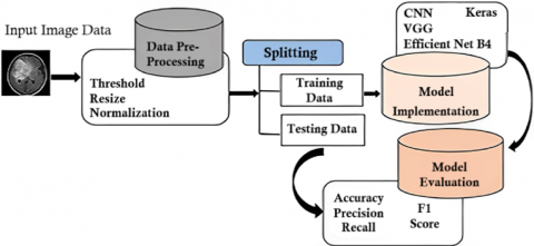
The methodology followed resembles the following sequence:
The methodology starts with importing necessary libraries into the environment. Then the next step is to set the paths for addressing the data imported into the drive. The process was carried out on Google’s Colab service, which provided the integration of Google Drive to import and use large datasets. Since the dataset exceeded the maximum limit allowed to be uploaded in the runtime, we had to mount google drive and import the data from there by specifying a path. Next comes the shuffling step so that the data for Yes and No (images containing tumor and not containing the tumor, respectively) do not group when training or testing the model. Then, the data is visualized using the imshow function from matplotlib, which allows us to read an image. The sample images of the dataset used for comparative implementation methodology is shown in Figure 1.
Figure 1. Dataset images of brain CT, MRI
Figure 2. Architecture diagram for non-diversified dataset based CNN
Figure 3. Architecture for diversified dataset based CNN
The next step was to split the data into training and testing. The training data size was 90%, with a random state seed value of 42. The next step was to generate data from images without diversification. From here on out, the proceeding methodology is divided into two sections, each following the same steps for diversified and non-diversified image data. The data was hence generated from the images. Next, as per Figure 2, the CNN model was to be developed for non-diversification. Firstly, the model structure was defined by having 4 2D convolutional layers with ReLU activation functions. Each was followed by a later 2 by 2 2D pooling and a dropout layer that removes any record with less than 20% recognition. Finally, a flattened layer was added with a dropout rate of 50% and two dense layers with ReLU and SoftMax activation functions, respectively. The model was then compiled using a loss rate of 0.001 and “Categorial Cross Entropy” as the loss function on the accuracy metric. Then the model fitting was carried out for 30 epochs with 120 steps each. The accuracy and other metrics were then checked by plotting them using matplotlib functions. Finally, the prediction score was calculated, and the prediction process was carried out.
Next, the data was generated from images with diversification as per Figure 3. All the steps were the same except for the structure of the CNN model, where we had 4 layers last time. We had 5 2D convolutional layers with ReLU activation function and only a pooling layer of 2 by 2 for each 2D convolutional layer. The dropout layer was put in at the end, along with dense layers. The flattening layer was added, followed by a dropout layer of 50% and two dense layers with ReLU and SoftMax activation functions, respectively. The rest of the process also remains identical to the previous section with only changes in the model fitting section, where we used 50 epochs with 122 steps in each epoch this time.
ConvOutput(x,y)=(FK*INP)(x,y)=∑∑FK(i,j)*INP(x+i,y+j) (1)
PoolingOutput(x,y)=Poo(INP[x*poolsize:(x+1)poolsize,y*poolsize:(y+1)poolsize]) (2)
DenseOutput=ActFun[(WeightMatrix*INP)+bias] (3)
whereas,
CNNOutput=Softmax(FullyConnected(Dense(FullyConnected(Dense(Flatten(MaxPooling2D(Conv2D(INP)))))))) (4)
Table 2. Architecture configuration of diversified and non-diversified CNN’s
|
Implementation Details |
Description (Model Architecture-Diversified & Non-Diversified CNN) |
|
Convolutional Layers |
Several convolutional layers with different filter sizes (32, 64, 128, 256) and “ReLu” activation. |
|
Max Pooling Layers |
Max pooling layers with pool size (2, 2) to down sample feature maps. |
|
Dropout Layers |
Dropout layers with a dropout rate of 0.2 for regularization and preventing overfitting. |
|
Flatten Layer |
Converts 2D feature maps to a 1D feature vector. |
|
Dense Layers |
Dense layers for classification after the flatten layer. |
|
Loss Function |
Categorical Crossentropy, suitable for multi-class classification problems. |
|
Batch Size |
Fit Function is Used. (Non-Diversified CNN). Batch size is 20 (Diversified CNN). |
|
Training |
Training is performed using the fit function with training data and validation data. |
|
Steps per Epoch |
120 steps per epoch, indicating the training data is divided into batches and processed accordingly. |
Figure 4. Workflow diagram for complete process of model architecture based on CNN-(diversified & non-diversified), EfficientNetB4, VGG-16 pre-processed Keras model
Table 3. Structure of developed model
|
Layer |
Description |
|
Base Model |
EfficientNetB4 with pre-trained weights from ImageNet, excluding the top layer. Input shape: img_shape |
|
Batch Normalization |
Normalizes the activations of the base model to improve training stability. |
|
Dense Layer |
Units: 256; Regularization: Kernel L2 (0.016), Activation L1 (0.006), Bias L1 (0.006); Activation: ReLU |
|
Dropout Regularization |
Rate: 0.45; Randomly drops out a fraction of units during training to prevent overfitting. |
|
Output Layer |
Dense layer with units equal to class_count (number of classes). Activation: Softmax |
|
Model Instantiation |
Inputs: base model input; Outputs: output layer |
|
Model Compilation |
Optimizer: Adamax; Learning Rate: 0.001; Loss: Categorical Cross-Entropy; Metric: Accuracy |
Table 2 outlines architecture configurations for diversified and non-diversified CNN models.
The TensorFlow Keras callbacks Reduce the Learning Rate on Plateau, Early Stopping, and Model Checkpoint are combined in the EfficientNetB4 [20]. Architecture, but some of their drawbacks are also addressed [21]. The base model used is EfficientNetB4 from the TensorFlow Keras applications. It is loaded with pre-trained weights from the ImageNet dataset and has its top layer (fully connected layer) excluded. The input shape of the model is specified as img_shape, which represents the shape of the input images. The output of the base model is passed through batch normalization, which helps normalize the activations and improve training stability. A Dense layer with 256 units is added using kernel regularization (L2 regularization with a coefficient of 0.016), activity regularization (L1 regularization with a coefficient of 0.006), and bias regularization (L1 regularization with a coefficient of 0.006). The activation function used for this layer is ReLU. Dropout regularization with a rate of 0.45 is applied to the previous layer, which helps prevent overfitting by randomly dropping out a fraction of the units during training.
The final output layer is a Dense layer with the number of units equal to class_count, representing the number of classes in the classification task. The activation function used is softmax, which produces probability distributions over the classes. The model is instantiated using the Model class, with the inputs set to the input of the base model and the outputs set to the output layer. The model is compiled using the Adamax optimizer with a learning rate 0.001. The loss function used is categorical cross-entropy, suitable for multi-class classification tasks. The accuracy metric is also specified for evaluation during training. The specific sizes of the convolution kernels in the EfficientNetB4 model are not explicitly specified. The EfficientNetB4 architecture consists of multiple convolutional layers with different kernel sizes defined internally within the EfficientNetB4 model implementation. The details of the mentioned model are given below in Table 3.
Additionally, it offers a summary of the model’s performance after each epoch that is simpler to understand. Further, it includes a valuable feature that allows us to select how many epochs we want to train for before receiving a message asking us to input H to cease training on the current epoch or an integer to define how many epochs we want to train for before hearing the message again. This is useful if we are developing a model and find that the metrics are suitable, and we want to halt the model training early. Remember that the callback always gives our model weights that have been changed to represent the epoch with the highest performance on the monitored metric (accuracy or validation accuracy). Figure 4 depicts a comprehensive workflow diagram encompassing the entire process of model architecture, which includes CNN-based models for both diversified and non-diversified datasets, as well as the pre-processed Keras models EfficientNetB4 and VGG-16.
The callback will keep track of training accuracy and change the learning rate accordingly until the accuracy meets a user-specified threshold level. Once that level of training accuracy is attained, the callback shifts to monitoring validation loss and modifies the learning rate accordingly. The callback has the following format:
“callbacks=[LRA(model, base_model, patience, stop_patience, threshold, factor, dwell, batches, initial_epoch, epochs, ask_epoch)]”
where:
The model using the fit function with several parameters and callbacks is trained with the number of epochs set to be 40, indicating that the model will undergo 40 complete passes through the training data during training. The patience parameter plays a role in adjusting the learning rate. It determines the number of epochs to wait before modifying the learning rate if the monitored value (either training accuracy or validation loss) does not improve. This parameter helps prevent premature adjustments to the learning rate. The stop_patience parameter specifies the number of epochs to wait before terminating the training process if the monitored value fails to improve. Once this threshold is reached, training will be halted. The threshold parameter defines the criteria for monitoring the performance metric. If the training accuracy falls below the threshold, the training accuracy itself will be used as the monitored value. However, if the training accuracy exceeds the threshold, the monitored value will be the validation loss. This dynamic selection allows for adaptive monitoring based on the training progress. The factor parameter determines the reduction factor applied to the learning rate when necessary. If the monitored value fails to improve, the learning rate will be decreased by this factor to fine-tune the model’s optimization process. The dwell parameter is a boolean flag that determines whether the model weights should revert to the weights from the previous epoch if the monitored metric does not show improvement. Enabling this flag can help prevent the model from getting stuck in a suboptimal state by reverting to a previously successful configuration. The freeze parameter, also a boolean flag, controls whether the weights of the base model should remain frozen during training. Freezing the base model allows for feature extraction while keeping the learned representations intact. The ask_epoch parameter specifies the frequency at which the user will be prompted to halt the training process. After running for the specified number of epochs, the training will pause and inquire if further training is desired. The batches parameter denotes the number of training batches to be processed per epoch. Batches are smaller subsets of the training data used for optimization, allowing for more efficient computation. The callbacks list includes a single callback object, LRA, which is an instance of a custom callback class. This LRA callback is responsible for dynamically adjusting the learning rate based on the specified criteria during training. It ensures that the learning rate adapts to the model’s performance, improving convergence. Finally, the training process commences using the fit function. The training generator (train_gen), validation generator (valid_gen), and other relevant parameters are passed to the function. The callbacks list is provided to enable learning rate adjustment and other functionalities during training, allowing for more effective and customized model optimization.
In summary, the provided model meticulously configures the parameters and callbacks required for training and then initiates the same using the fit function, incorporating the specified parameters and the LRA callback to facilitate learning rate adjustments. This comprehensive approach ensures an efficient and adaptive training process, ultimately leading to improved model performance.
This relationship is summarized as follows:
The learning rate adjustment occurs iteratively throughout the training process, with the LRA class incorporating various variables and calculations to quantify the relationship. These include self.count, self.patience, self.stop_count, self.stop_patience, self.highest_tracc, self.lowest_vloss, and self.factor. These parameters and calculations influence how the learning rate changes in response to training accuracy and validation loss.
To gain a more comprehensive understanding of the learning rate trend and its relationship with training accuracy, it is recommended to examine the training history and the information printed during training. This includes monitoring the changes in learning rate, accuracy, validation loss, and epoch progression. By analyzing this information, one can gain insights into the dynamics of the learning rate and its impact on the training process. From the provided output in Figure 5 and Figure 6, we can analyze the trend of the learning rate throughout the training process.
Initially, the learning rate is set to 0.001. The training starts with an epoch of 1, where the loss is 6.143, accuracy is 90.375%, validation loss is 4.55959, and validation accuracy is 97.667%. As the training progresses, we observe a consistent learning rate of 0.001, and the monitored metric is the validation loss. During the first few epochs, the validation loss experiences fluctuations. However, after epoch 10, the training continues until epoch 21, as indicated by the user input. At this stage, the learning rate remains unchanged at 0.001.
Figure 5. Ask_epoch function depicting epoch initialization count
Figure 6. “H” option to halt training & integer input to continue
From epoch 22 onwards, the learning rate transitions to 0.0005 based on the specified adjustment factor. The monitored metric remains the validation loss. The training continues until epoch 40, where the learning rate further decreases to 0.00013. Throughout this phase, the validation loss shows a decreasing trend, indicating improvement in the model’s performance. It is noteworthy that the validation accuracy remains consistently high at 100% throughout the entire training process, demonstrating the model’s ability to generalize well to unseen data.
In summary, the learning rate follows a pattern of adjustment based on the specified factors and the monitored validation loss. It gradually decreases as the training progresses, suggesting a fine-tuning of the model’s optimization process. This adaptive adjustment ensures that the model converges towards a better solution in the parameter space, leading to improved performance.
In observation, the article discusses several strategies to address the challenge of training with a limited number of samples. These techniques include data augmentation, leveraging pre-trained models through transfer learning, regularization methods, early stopping, and learning rate adjustment. Data augmentation expands the training dataset by applying various transformations to the available samples, reducing overfitting. Transfer learning allows the utilization of pre-trained models trained on large-scale datasets to leverage their knowledge for the specific task at hand. Regularization techniques, such as dropout and weight regularization, help prevent overfitting and improve model generalization. Early stopping stops the training process if no improvement is observed, preventing overfitting on limited data. Learning rate adjustment dynamically adjusts the learning rate to optimize model convergence. By employing these techniques collectively, the article addresses the challenge of few-sample training and enhances the performance of the model with a limited training dataset.
In this section, we provide an overview of the hardware and software specifications utilized in our experiments.
Table 4. Prediction metrics for diversified and non-diversified data
|
Component |
Manufacturer & Version |
Size |
|
Processor |
Intel Core i7, 10870@2.20 Ghz |
NA |
|
RAM |
DDR4-Speed 2667 Mhz |
16GB |
|
GPU1 |
Intel Iris-XE Graphics |
Shared up to 8 GB |
|
GPU2 |
Nvidia GeForce GTX 1650 Ti |
Dedicated 4 GB, Shared up to 8 GB |
|
GPU3 |
Google Colab Shared GPU T4 |
NA |
|
Operating System |
Windows 11 |
NA |
|
Environment Used |
Google Colab Python Virtual Environment |
NA |
|
Packages/Libraries used. |
|
|
|
Input to model |
|
|
The experimental setup used for the analysis is represented in Table 4. The study was divided into two sections-the data was derived from images without and with diversifications in the respective order. After training the model, the results are analyzed in two main metrics-Loss and Prediction accuracy [22, 23] for both sections, which are mentioned below in Table 5. Table 6 is a comparison of accuracies recorded by existing methods with diversified and non-diversified data models.
Table 5. Prediction metrics for diversified and non-diversified data
|
S. No. |
Metrics of predictions |
||
|
Particulars |
Loss |
Accuracy |
|
|
1. |
Non-Diversified Data-CNN |
26% |
97% |
|
2. |
Diversified Data-CNN |
25% |
89% |
|
3. |
EfficientNetB4 |
<1% |
99.67% |
|
4. |
VGG Architecture-16 Using Keras Pre-Processed Models |
<23% |
96% |
Table 6. Prediction metrics for comparison b/w existing models & CNN’s diversified and non-diversified data model
|
Accuracy Predictions Based on Comparison |
||||
|
Particulars |
Their Accuracy |
Our Accuracy (With/Without Diversification of CNN Model) |
EfficientNetB4 |
Keras Pre-Processed VGG Architecture |
|
Deepak and Ameer (CNN Model without Transfer Learning) |
84.19% |
97% & 89% |
99.67% |
96% |
|
Amin et al. (“Multi-Layer Perceptron”) |
Average B/w 88.20% to 96.70% |
97% & 89% |
99.67% |
96% |
|
Sharma et. al. (GLCM using Naïve Bayes) |
MLP 98.60% Naïve Bayes 91.60% |
97% & 89% |
99.67% |
96% |
|
Zulpe and Pawar (“Grey Level Concurrence Matrix”) |
Classification Rate: -97.5% |
97% & 89% |
99.67% |
96% |
|
Hussein et al. (3D CNN) |
91.26% |
97% & 89% |
99.67% |
96% |
|
Yang et al. (GoogleNet & AlexNet) |
90.90% Test Accuracy |
97% & 89% |
99.67% |
96% |
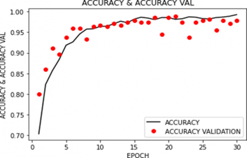
In Figure 7, we present accuracy metrics obtained from the evaluation of our implemented models, including the EfficientNetB4 model and a customized CNN architecture. For CNN, the first section for non-diversified data, Figure 8, shows the plot for model accuracy in blue and accuracy for validation data set in orange on the vertical axis plotted against several epochs on the horizontal axis.
Figure 9 shows the value of the loss function in black and the loss for validation data set in red circles on the vertical axis plotted against several epochs on the horizontal axis.
Figure 10 shows the value for accuracy and accuracy for validation data set in red circles on the vertical axis plotted against the number of epochs on the horizontal axis.
Figure 11 shows the value for loss and validation data loss, accuracy, and validation data accuracy, all in one chart on the vertical axis plotted against the number of epochs on the horizontal axis.
Figure 7. Accuracy metrics for efficientnetb4 model & CNN architecture
Figure 8. Plot for accuracy and validation accuracy against a number of epochs
Figure 9. Plot for accuracy and validation accuracy against a number of epochs
Figure 10. Plot for accuracy and validation accuracy against a number of epochs
Figure 11. Plot for loss and validation loss, accuracy, and validation accuracy against the number of epochs
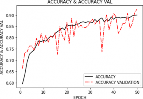
For the second section for diversified data, Figure 12 shows the plot for model accuracy in blue and the accuracy for validation data set in orange on the vertical axis plotted against the number of epochs on the horizontal axis.
Figure 13 shows the value for loss in a solid black line and validation data loss in a dashed red line on the vertical axis plotted against the number of epochs on the horizontal axis.
Figure 14 shows the accuracy value in the solid black line and validation data accuracy in the dashed red line on the vertical axis plotted against the number of epochs on the horizontal axis.
Figure 12. Plot for loss and validation loss, accuracy, and validation accuracy against the number of epochs
Figure 13. Plot for loss and validation loss against a number of epochs
Figure 14. Plot for loss, accuracy, validation loss, and validation accuracy
Figure 15. Plot for loss, validation loss, and accuracy, validation accuracy plotted against the number of epochs
Figure 15 shows the value of the loss, validation loss, and accuracy, validation accuracy combined in a single plot on the vertical axis plotted against the number of epochs on the horizontal axis.
For EfficientNetB4, The Total Epochs are 40, Total Training Time elapsed is 1 Hour 33 Minutes 44.97 Seconds. The Accuracy is 99.67% & The Loss is <1%. Figure 16 displays the training and validation loss curves for our implemented EfficientNetB4 model. These curves illustrate how the model's loss changes over a varying number of training epochs.
Figure 16. Plot for loss and validation loss against a number of epochs for EfficientNetB4
In Figure 17, we present the training and validation accuracy curves for the EfficientNetB4 model. These curves provide valuable insights into the model's learning progress and its ability to generalize to unseen data as training progresses.
Figure 18 showcases the confusion matrix for the EfficientNetB4 model. The F1 Score of 1 indicates a perfect balance between precision and recall.
Figure 19 demonstrates the training and validation accuracy curves for the Keras pre-processed VGG model. These curves reveal how well the model learns and generalizes across various epochs, aiding in the assessment of its effectiveness for the specific task.
Figure 17. Plot for accuracy and validation accuracy against a number of epochs for EfficientNetB4
Figure 18. Confusion matrix for EfficientNetb4 model: -F1 Score=1
Figure 19. Plot for accuracy and validation accuracy against a number of epochs for the Keras pre-processed VGG model
Figure 20 illustrates the training and validation loss curves for the Keras pre-processed VGG model which is crucial for understanding the model's convergence.
The EfficientNetB4 model achieved an F1 score on the test set of 100% [24]. There was 1 misclassification in 300 test images.
The Keras Pre-Processed Model-VGG Architecture results comprise 90-96% accuracy.
Figure 20. Plot for loss and validation loss against a number of epochs for the Keras pre-processed VGG Model
This study aims to present an automatic and accurate model for predicting and detecting the presence of brain tumors in MRI scan images with minimal pre-processing required. The performance was evaluated on metrics of accuracy and loss. The model achieved 97% on non-diversified data and 89% on diversified data, even 99.67% accuracy by EfficientNETB4, but still, many improvements are possible. Firstly, the data could be increased to be more inclusive of different images to improve the model’s accuracy on the unseen data set. Secondly, further improvements in the feature extraction methods can be made, and more accurate and efficient techniques can be applied for the extraction of features. Other work in this area shall help address these issues, probably using transfer learning concepts [25].
As with any study conducted, there is always room for improvements and further advancements. In this context, the accuracy achieved using neural networks can be further improved by incorporating transfer learning models in a better way. The use of deep learning techniques to include further detailed classification possibilities, such as segmenting the regions with sub-tumoral growth that have complete, core, and enhanced tumors from the images and this, can be further extended to achieve even better accuracy and usability of machine learning in the field of prediction of medical conditions using imagery.
In several qualitative and quantitative comparisons, the proposed deep learning-based model of brain tumor identification outperforms previously published models. The model is more robust to employ in a variety of scenarios because it was trained on a diversified dataset. As noted in the results section, this model would also be simple to adapt to and capable of producing higher accuracy compared to previous models. It was discovered that the proposed framework spontaneously adopted features during training, and it has demonstrated outstanding generalization abilities, correctly identifying brain tumors in uncommon and difficult instances. This model can be scaled for usage with datasets of greater size.
To support our claims, we ran an experiment in which we compared our results to those of other approaches already in use, using benchmark datasets and assessment criteria that are widely used in the field of brain tumor identification. To demonstrate the superiority of our deep learning model, comparative studies have concentrated on the accuracy, computational efficiency, interpretability, and generalization.
[1] Zhang, J.C., Shen, X.L., Zhuo, T.Q., Zhou, H. (2017). Brain tumor segmentation based on refined fully convolutional neural networks with a hierarchical dice loss. arXiv Preprint arXiv: 1712.09093. https://doi.org/10.48550/arXiv.1712.09093
[2] Seetha, J., Raja, S.S. (2018). Brain tumor classification using convolutional neural networks. Biomedical & Pharmacology Journal, 11(3): 1457-1461. https://doi.org/10.13005/bpj/1511
[3] https://www.cancer.net/cancer-types/brain-tumor/statistics, accessed on 20 July 2023.
[4] Shao, L., Zhu, F., Li, X.L. (2014). Transfer learning for visual categorization: a survey. IEEE Transactions on Neural Networks and Learning Systems, 26(5): 1019-1034. https://doi.org/10.1109/TNNLS.2014.2330900
[5] Zacharaki, E.I., Wang, S.M., Chawla, S., Soo Yoo, D., Wolf, R., Melhem, E.R., Davatzikos, C. (2009). Classification of brain tumor type and grade using MRI texture and shape in a machine learning scheme. Magnetic Resonance in Medicine: An Official Journal of the International Society for Magnetic Resonance in Medicine, 62(6): 1609-1618. https://doi.org/10.1002/mrm.22147
[6] Deepak, S., Ameer, P.M. (2019). Brain tumor classification using deep CNN features via transfer learning. Computers in Biology and Medicine, 111: 103345. https://doi.org/10.1016/j.compbiomed.2019.103345
[7] Zulpe, N., Pawar, V. (2012). GLCM textural features for brain tumor classification. International Journal of Computer Science Issues (IJCSI), 9(3): 354-359.
[8] Sharma, K., Kaur, A., Gujral, S. (2014). Brain tumor detection based on machine learning algorithms. International Journal of Computer Applications, 103(1): 7-11. https://doi.org/10.5120/18036-6883
[9] Mohsen, H., El-Dahshan, E.S.A., El-Horbaty, E.S.M., Salem, A.B.M. (2018). Classification using deep learning neural networks for brain tumors. Future Computing and Informatics Journal, 3(1): 68-71. https://doi.org/10.1016/j.fcij.2017.12.001
[10] Bauer, S., May, C., Dionysiou, D., Stamatakos, G., Buchler, P., Reyes, M. (2011). Multiscale modeling for image analysis of brain tumor studies. IEEE Transactions on Biomedical Engineering, 59(1): 25-29. https://doi.org/10.1109/TBME.2011.2163406
[11] Islam, A., Reza, S.M.S., Iftekharuddin, K.M. (2013). Multifractal texture estimation for detection and segmentation of brain tumors. IEEE Transactions on Biomedical Engineering, 60(11): 3204-3215. https://doi.org/10.1109/TBME.2013.2271383
[12] Deniz, E., Şengür, A., Kadiroğlu, Z., Guo, Y.H., Bajaj, V., Budak, Ü. (2018). Transfer learning based histopathologic image classification for breast cancer detection. Health Information Science and Systems, 6: 1-7. https://doi.org/10.1007/s13755-018-0057-x
[13] Hussein, S., Kandel, P., Bolan, C.W., Wallace, M.B., Bagci, U. (2019). Lung and pancreatic tumor characterization in the deep learning era: novel supervised and unsupervised learning approaches. IEEE Transactions on Medical Imaging, 38(8): 1777-1787. https://doi.org/10.1109/TMI.2019.2894349
[14] Yang, Y., Yan, L.F., Zhang, X., Han, Y., Nan, H.Y., Hu, Y.C., Hu, B., Yan, S.L., Zhang, J., Cheng, D.L., Ge, X.W., Cui, G.B., Zhao, D., Wang, W. (2018). Glioma grading on conventional MR images: A deep learning study with transfer learning. Frontiers in Neuroscience, 12: 804. https://doi.org/10.3389/fnins.2018.00804
[15] Natarajan, P., Krishnan, N., Kenkre, N.S., Nancy, S., Singh, B.P. (2012). Tumor detection using threshold operation in MRI brain images. In 2012 IEEE International Conference on Computational Intelligence and Computing Research, IEEE, pp. 1-4. https://doi.org/10.1109/ICCIC.2012.6510299
[16] Joshi, D.M., Rana, N.K., Misra, V.M. (2010). Classification of brain cancer using artificial neural network. In 2010 2nd International Conference on Electronic Computer Technology, IEEE, pp. 112-116. https://doi.org/10.1109/ICECTECH.2010.5479975
[17] Amin, S.E., Megeed, M.A. (2012). Brain tumor diagnosis systems based on artificial neural networks and segmentation using MRI. In 2012 8th International Conference on Informatics and Systems (INFOS), MM-119.
[18] Goswami, S., Bhaiya, L.K.P. (2013). Brain tumour detection using unsupervised learning based neural network. In 2013 International Conference on Communication Systems and Network Technologies, IEEE, pp. 573-577. https://doi.org/10.1109/CSNT.2013.123
[19] George, E.B., Karnan, M. (2012). MRI brain image enhancement using filtering techniques. International Journal of Computer Science & Engineering Technology (IJCSET), 3(9): 399-403.
[20] Nalwar, S., Shah, K., Bidwe, R.V., Zope, B., Mane, D., Jadhav, V., Shaw, K. (2022). EffResUNet: encoder decoder architecture for cloud-type segmentation. Big Data and Cognitive Computing, 6(4): 150. https://doi.org/10.3390/bdcc6040150
[21] Bidwe, R.V., Mishra, S., Patil, S., Shaw, K., Vora, D.R., Kotecha, K., Zope, B. (2022). Deep learning approaches for video compression: a bibliometric analysis. Big Data and Cognitive Computing, 6(2): 44. https://doi.org/10.3390/bdcc6020044
[22] Bidwe, S., Kale, G., Bidwe, R. (2022). Traffic monitoring system for smart city based on traffic density estimation. Indian Journal of Computer Science and Engineering, 13(5): 1388-1400. https://doi.org/10.21817/indjcse/2022/v13i5/221305006
[23] Mane, D., Bidwe, R., Zope, B., Ranjan, N. (2022). Traffic density classification for multiclass vehicles using customized convolutional neural network for smart city. In Communication and Intelligent Systems: Proceedings of ICCIS, Singapore: Springer Nature Singapore, 2021: 1015-1030. https://doi.org/10.1007/978-981-19-2130-8_78
[24] Mane, D., Shah, K., Solapure, R., Bidwe, R., Shah, S. (2022). Image-based plant seedling classification using ensemble learning. In Proceedings of the 6th International Conference on Advance Computing and Intelligent Engineering (ICACIE), Singapore: Springer Nature Singapore, 2021: 433-447. https://doi.org/10.1007/978-981-19-2225-1_39
[25] Zope, B., Mishra, S., Shaw, K., Vora, D.R., Kotecha, K., Bidwe, R.V. (2022). Question answer system: a state-of-art representation of quantitative and qualitative analysis. Big Data and Cognitive Computing, 6(4): 109. https://doi.org/10.3390/bdcc6040109