Balasundaram Gopi*![]() | James Visumathi
| James Visumathi![]() | Sampath Jayanthi
| Sampath Jayanthi![]() | Shaik Mahaboob Basha
| Shaik Mahaboob Basha![]()
© 2023 IIETA. This article is published by IIETA and is licensed under the CC BY 4.0 license (http://creativecommons.org/licenses/by/4.0/).
OPEN ACCESS
In this study, we propose a Second Order Shearlets (SOS) based system for Oral Cancer Classification (OCC) that leverages histopathological images. The fundamental premise of the system is the observable variations in texture patterns between normal and abnormal cells within these images, which can be exploited for differentiation. The images undergo a transformation from the Red-Green-Blue (RGB) color space to the Hue-Saturation-Value (HSV) color space, followed by the extraction of co-occurrence texture features via the SOS system. Further enhancement of feature extraction is achieved by applying a median filter for de-noising the histopathological images. The proposed SOS-OCC system, equipped with a probabilistic classifier at the final stage, was presented with an assortment of 1224 images for evaluation. The results indicated a noteworthy classification accuracy of 98.6% when employing stratified k-fold cross-validation, thereby underlining the system's efficacy in identifying oral cancer-related abnormalities. Moreover, a comparative analysis was conducted with Wavelet, Curvelet, and Contourlet-based representation systems to underscore the superior performance of the SOS-OCC system. This study provides valuable insights into the application of the SOS approach to oral cancer classification and sets a promising precedent for future research.
oral cancer, multi-scale analysis, multi-directional analysis, Second Order Shearlets, colour spaces
Oral cancer, a result of cellular mutations within the oral cavity, manifests a higher incidence in males compared to females. Risk factors include smoking, excessive alcohol consumption, a sub-optimal diet, and a familial history of cancer. Early diagnosis enhances survival rates, thus necessitating the development of effective classification systems [1].
Prior studies have focused on various aspects of Oral Cancer Classification (OCC) systems. For instance, one utilized temporal features, energy, and entropy components from each color channel of median filtered histopathological images, employing k-nearest neighbors and support vector machine classifiers for OCC [1]. Another study implemented a Convolutional Neural Network (CNN) based OCC system with optimally adjusted layers and filters for high performance extraction of deep features [2]. Efforts to reduce computational complexity led to the development of a lightweight CNN model with fewer parameters [3], while an attention-based CNN system was designed to offer two paths for efficient classification: compression and learning [4].
In addition to these, the literature also presents OCC systems that employ a fuzzy Support Vector Machine (SVM) [5], a multiple instance learning-based approach [6], and asymmetric residual hash-based histopathological image retrieval [7]. Other studies have focused on the development of a matrix form classifier [8], dictionary learning for histological image classification [9], an auto-encoder based system [10], and a feature blending approach [11]. Spatial and morphological methods have also been explored [12], as have adaptive fuzzy systems [13], trust counting-based systems [14], and the use of a golden eagle optimization algorithm for feature selection [15]. Furthermore, the influence of dimensionality within CNN has been examined [16].
In light of the aforementioned studies, the present work aims to explore the extraction of textures from histopathological images using Second Order Shearlets (SOS) for OCC. The proposed approach involves the use of co-occurrence features of SOS sub-bands for the discrimination between normal and abnormal images.
The remainder of the paper is structured as follows: Section 2 elaborates on the design of the SOS-based OCC system, while Section 3 presents a comparative analysis of the SOS-OCC system's results with those of Wavelet [17], Curvelet [18], Contourlet [19], and First Order Shearlets (FOS) based systems. Finally, Section 4 provides a conclusion, drawing upon the experimental results.
The structures within the histopathological images may give rise to either low-level or high-level textures. In many cases, such textures are influenced by disease processes. The proposed SOS for the OCC system is considered a binary pattern recognition system with three stages; preprocessing, feature extraction, and probabilistic classification. Figure 1 shows the block diagram of the SOS based OCC system.
Figure 1. Proposed SOS-OCC system using histopathological images
2.1 Preprocessing
This is the first stage of the SOS-OCC system where noise removal and colour space conversion occur. A median filter, which is a non-linear filter, is employed to remove noise and preserve edges [1]. This study uses a small window of 3×3 and finds the median value inside the window. The center pixel is replaced by the median value to restore the noise-free pixel. This process is repeated until the last pixel is restored. It is an order statistic filter that operates on the data inside a window of size (2m+1, 2m+1). It is defined by
$\begin{array}{r}M F_{i j}=\operatorname{median}\left\{I_{i+k, j+l}: k, l=-m, \ldots m\right\} \\ \text { for } i, j=(m+1) \ldots . .(n-m)\end{array}$ (1)
where, the noisy image is represented as I and the pixel’s location are (i,j). Figure 2(a) shows the histopathological images and Figure 2(b) shows its corresponding noise free images.
After noise removal, RGB to HSV (Hue, Saturation, and Value) colour space conversion takes place. The HSV colour space aligns with the human vision more closely than the RGB colour space. It represents the models in such a way that how colour appears under the light. The conversion formulae [20] are as follows:
$\begin{array}{r}H=\cos ^{-1} \frac{0.5[(R-G)+(R-B)]}{\sqrt{(R-G)^2+(R-B)(G-B)}} \\ H \in[0, \pi] \text { for } B \leq G\end{array}$ (2)
$\begin{array}{r}H=2 \pi-\cos ^{-1} \frac{0.5[(R-G)+(R-B)]}{\sqrt{(R-G)^2+(R-B)(G-B)}} \\ H \in[\pi, 2 \pi] \text { for } B \succ G\end{array}$ (3)
$S=1-\frac{3}{R+G+B} \min (R, G, B)$ (4)
$I=\frac{R+G+B}{3}$ (5)
where, H, S, and V represent the Hue, Saturation and Value components in the HSV colour space corresponding to R (Red), G (Green), and B (Blue) components in the RGB colour space. Figure 3(a) shows the HSV images of RGB images in Figure 2(b) and the components of HSV colour spaces are shown in Figure 3(b) to Figure 3(d).
Figure 2. (a) Input histopathological images (b) Noise free images by median filter
Figure 3. (a) HSV images of RGB images in Figure 2(b); (b) H channel; (c) S channel; (d) V channel
2.2 Feature extraction
In this stage, a perception-based statistical method is employed to extract histopathological images' features. The 1st order stochastic features are based on the Probability Density Function (PDF) distribution of intensities. In contrast, the 2nd order features are obtained from the PDF of pairs of intensity levels. The co-occurrence features are based on the estimation of the 2nd order joint PDF f(i,j|Δx,Δy) where the spacing between the pair of pixel (i,j) in the x and y directions are represented by Δx and Δy respectively. It is defined for an input image I of size NxN.
$C_{\Delta(i, j)}=\frac{\#(((x, y),(x+\Delta x, y+\Delta y)): I(x, y)=i, I(x+\Delta x, y+\Delta y)=j)}{\#(((x, y),(x+\Delta x, y+\Delta y)): 1 \leq x, y, x+\Delta x, y+\Delta y) \leq N}$ (6)
The application of Eq. (6) produces a co-occurrence matrix from which a number of stochastic texture features can be computed. To compute the co-occurrence matrix, the frequency of occurrence of a pixel with intensity i adjacent to a pixel with intensity j is generated for all elements (i,j) of the given square matrix. Then the normalized co-occurrence matrix is obtained by dividing all elements in the co-occurrence matrix by the total number of frequency of occurrences. Due to the normalization, the sum of all elements in the co-occurrence matrix equals 1. There are 14 features [21] that can be extracted and are undoubtedly the most well-known features used in many texture analysis methods in the medical domain. Table 1 shows the extracted texture features.
Table 1. SOS-OCC system's performance measures
|
No |
Features |
No |
Features |
|
1 |
Contrast |
8 |
Angular second Moment |
|
2 |
Sum of Squares (Variance) |
9 |
Correlation |
|
3 |
Sum Average |
10 |
Inverse different moment |
|
4 |
Entropy |
11 |
Sum Variance |
|
5 |
Difference Variance |
12 |
Difference Entropy |
|
6 |
Sum Entropy |
13 |
Maximal Correlation Coefficient |
|
7 |
Information Measures of Correlation-1 |
14 |
Information Measures of Correlation-2 |
Before feature extraction, each component of HSV image is represented by SOS [22, 23]. From the obtained SOS sub-bands, the stochastic texture features are extracted. The SOS is defined by
$\psi_{c s t}(x)=\frac{1}{\left|\operatorname{det} P_{s d}\right|} \Psi\left(P_{s d}^{-1}(x-t)\right)$ (7)
where, Psd is the product of SOS operator and dilation matrices. They are defined in Eq. (8) and Eq. (9) respectively.
$S_r^{(l)}(x):=\left(\begin{array}{cc}1 & \sum_{m=1}^l r_m x_2^{m-1} \\ 0 & 1\end{array}\right)\left(x_1, x_2\right)^T$ (8)
$A_{a, \alpha}=\left(\begin{array}{cc}a & 0 \\ 0 & a^\alpha\end{array}\right)$ where $a>0$ and $\alpha \in[0,1]$ (9)
where, α is the scaling factor and $\alpha=\frac{1}{3}$ is used to analyze the SOS for OCC. This scaling helps to identify the location and the direction of discontinuity curves. For frame construction, the decomposition system employs some form of anisotropy. The orientation and location of system elements are controlled by the constructed frames. Ridgelet transform uses α=0, wavelet transforms use α=1 and the Curvelet and Shearlets use α=0.5. These values are not sufficient for separating different curvatures by the SOS that requires $0<\alpha<\frac{1}{2}$. The rates of decay vary depending on the circumstances, which in turn makes it possible to locate the boundaries. Using this scaling with $\alpha=\frac{1}{3}$, the decay rate of SOS offers more precise curvature and orientations of distinct areas in an image [23]. Figure 4 shows samples of 3rd level sub-bands of different representation systems. Features are extracted from each channel of the HSV colour space. From each sub-band, a total of 42 features are extracted per sample.
Figure 4. Sub-bands at 3rd level decomposition (a) SOS (b) FOS (c) Contourlet (d) Curvelet (e) Wavelet
2.3 Probabilistic classification
The probabilistic classifiers compute the possibilities of samples that may fall into one or more classes. The Bayesian classifier performs better in many medical image classification systems than the probabilistic classifiers. Using the posterior probabilities, the Bayesian classifier classifies whether the sample belongs to normal or abnormal. Let us consider the test sample as s. The Bayesian classifier is defined by
$\left\{\begin{array}{l}P\left(\omega_1 \mid s\right)>P\left(\omega_2 \mid s\right), \text { normal } \\ P\left(\omega_1 \mid s\right)<P\left(\omega_2 \mid s\right), \text { abnormal }\end{array}\right.$ (10)
where, $P\left(\omega_1 \mid s\right)$ and $P\left(\omega_2 \mid s\right)$ denote the posterior probabilities of belonging to normal and abnormal respectively. These probabilities can be obtained using Bayesian theorem and are given by:
$P\left(\omega_1 \mid s\right)=\frac{P\left(\omega_1\right) P\left(\omega_1 \mid s\right)}{P(s)}$ (11)
$P\left(\omega_2 \mid s\right)=\frac{P\left(\omega_2\right) P\left(\omega_2 \mid s\right)}{P(s)}$ (12)
Suppose the prior probability P(ω1) and P(ω2) are equal to each other. The Bayesian classifier in Eq. (9) can be yielded as:
$\left\{\begin{array}{l}P\left(s \mid \omega_1\right)>P\left(s \mid \omega_2\right), \text { normal } \\ P\left(s \mid \omega_1\right)<P\left(s \mid \omega_2\right), \text { abnormal }\end{array}\right.$ (13)
Thus, the classification depends on the comparison between $P\left(s \mid \omega_1\right)$ and $P\left(s \mid \omega_2\right)$.
The power of texture to discriminate oral cancer patients from normal subjects is accessed from 1224 (290 normal and 934 abnormal) histopathological images [24]. Figure 5 shows the histopathological images of normal and abnormal categories. As the resolutions of images in the databases are not equal, the resolution of images is set to 256×256 pixels after median filtering. In order to represent the images in SOS, Wavelet, Curve let, and Contourlet, a square-shaped resolution (256×256) is chosen.
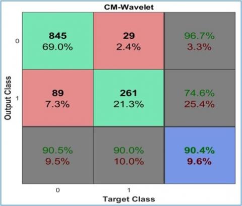
The commonly used model evaluation approaches are train/test split and k-fold cross-validation. Though they are very effective, they provide misleading results when used on an imbalanced database. As the database is imbalanced (290 normal and 934 abnormal), stratified k-fold cross-validation is employed. It is an extension of the standard k-fold cross-validation. The standard approach divides the dataset into k-folds, but it does not ensure that each fold has the same number of images per category. In contrast to the standard approach, the stratified approach maintains the same number of images per category in each sub-set. In this approach, stratified 10-fold cross-validation is employed. Thus, each fold has 29 normal and 93 abnormal samples. The remaining four abnormal samples from 934 samples are added in the last four-folds. The SOS-OCC system’s performance measures are shown in Table 2 and the confusion matrices obtained by the features are shown in Figure 6. In Figure 6, zero (0) represents the abnormal class and one (1) represents the normal class.
It is inferred from Figure 6 that the SOS-OCC system performs significantly better than others, with an overall accuracy of 98.6%. The sensitivity and specificity of the SOS-OCC system are 99.1% and 96.9%, respectively. The accuracies of other systems are 95.4% (Contourlet), 93% (Curvelet), and 90.4% (Wavelet). The obtained texture features from histopathological images contribute to significant performance improvement. Texture features from other transformations such as wavelet and contour let are insufficient to significantly discriminate the normal and abnormal tissues, thus their performances are less than the SOS based system. Figure 7 shows the OCC system's ROCs by different representation systems. In Figure 7, true positive rate is the positive prediction rate (sensitivity) of the system, whereas the false positive rate is the incorrect prediction of positive classes (1-specificity).
The most striking feature of all ROCs is how they are very close to the y-axis. Based on this feature, the ROC curve is interpreted. The two ends of the curve correspond to situations in which all states are considered to be normal (specificity=0 and sensitivity=1), or all states are considered to be pathological (specificity=1 and sensitivity=0), respectively. The points in the middle represent different degrees of decision making that are intermediate in nature. The ROC curve of a perfect observer, who never makes an incorrect diagnosis, will look like a step-by-step function, with axes that are labeled x=0 and y=1, whereas the ROC curve of a chance observer, who randomly diagnoses each case as normal or abnormal, will look like a straight line with a gradient of one that passes through the origin. If the ROC is located closer to the top left corner of the graph, then one observer is superior than the other (0.1 point). So, this provides a framework by which to compare the observations of many witnesses (in this case, automated techniques). The ROC curves for each observer may be derived, and then a comparison can be made by selecting (as the best observer) the curve that is located in the area of the graph that is most directly above the top left corner.
As this curve is drawn between the sensitivity and 1-specificity, the curve for the system very close to the y-axis is the best compared to others. Thus, the best system for OCC is in the order of SOS>FOS>Contourlet>Curvelet>Wavelet. All the performance measures shown in Figure 6 and Figure 7 are obtained by decomposing the histopathological images at 3-level with 8-directions. Figure 8 shows the performance for other levels of decomposition.
Figure 5. Sample histopathological images
Table 2. SOS-OCC system's performance measures
|
Sensitivity (%) |
Specificity (%) |
Overall Accuracy (%) |
|
True Positive (TP) |
True Negative (TN) |
TP+TN |
|
True Positive (TP)+True Negative (FN) |
False Positive (FP)+True Negative (TN) |
TP+FP+TN+FN |
Table 3. SOS-OCC system's performance for different validation approaches
|
Techniques |
System Accuracy (%) |
||
|
Random Split (70:30) |
k-fold Cross Validation (k=10) |
stratified k-fold Cross Validation (k=10) |
|
|
Wavelet |
84.5 |
86.8 |
90.4 |
|
Curvelet |
88.5 |
90 |
93.0 |
|
Contourlet |
90.8 |
92.6 |
95.4 |
|
FOS |
93 |
94.8 |
96.4 |
|
SOS |
95.7 |
96.5 |
98.6 |
(a) Wavelet
(b) Curvelet
(c) Contourlet
(d) FOS
(e) SOS
Figure 6. Confusion matrices of the OCC system using different representation systems
It can be seen from Figure 8 that the features from the 3rd level of representation systems provide better results than the other levels. This is because low-level features cannot distinguish the patterns of normal and abnormal images. While increasing the level from 1 to 2 and then to 3, the system’s accuracy increases as more discriminating features are extracted. However, the system’s accuracy decreases due to the redundant data at higher levels [25]. Among the representation systems, the performance of Wavelet is poorer as it provides only three directional features such as diagonal, vertical and horizontal.
Table 3 shows the performance of stratified k-fold cross-validation approach with other validation approaches such as random split (70:30) and k-fold cross-validation in terms of accuracy using 3rd level features from each representation systems. It can be seen from Table 3 that the stratified k-fold cross-validation approach gives better results than other validation approaches. This is because the stratified k-fold cross-validation is better for imbalanced dataset.
Figure 7. OCC system's ROCs by different representation systems
Figure 8. OCC system's performances for different levels
The texture changes in the histopathological images are significant in interpreting them to achieve high classification accuracy. In this work, an SOS based OCC system is designed using histopathological images. The texture differences between the abnormal and normal histopathological images are assessed using 1224 images obtained from oral cancer patients. The resulting 2nd order stochastic texture feature achieved a classification accuracy of 98.6% (Sensitivity 99.1% and specificity 96.9%) using a Bayesian classifier. The results proved that the SOS-OCC system might have applications in the early detection of oral cancer. The performance of the stochastic texture features is analyzed using different frequency domain representation systems such as Wavelet, Curvelet, Contourlet, FOS, and SOS. The obtained accuracies are 96.4% (FOS), 95.4% (Contourlet), 93% (Curvelet) and 90.4% (Wavelet). In the future, the specificity of the SOS-OCC system can be improved by using a balanced database while training and testing the classifier.
[1] Bakare, Y.B., Kumarasamy, M. (2021). Histopathological image analysis for oral cancer classification by support vector machine. International Journal of Advances in Signal and Image Sciences, 7(2): 1-10. https://doi.org/10.29284/ijasis.7.2.2021.1-10
[2] Archana, P., Megala, T., Udaya, D., Prabavathy, S. (2021). Classification of histopathological variants of oral squamous cell carcinoma using convolutional neural networks. In Big Data Management in Sensing, pp. 1-14.
[3] Kumar, A., Sharma, A., Bharti, V., Singh, A.K., Singh, S.K., Saxena, S. (2021). MobiHisNet: A lightweight CNN in mobile edge computing for histopathological image classification. IEEE Internet of Things Journal, 8(24): 17778-17789. https://doi.org/10.1109/JIOT.2021.3119520
[4] Brancati, N., De Pietro, G., Riccio, D., Frucci, M. (2021). Gigapixel histopathological image analysis using attention-based neural networks. IEEE Access, 9: 87552-87562. https://doi.org/10.1109/ACCESS.2021.3086892
[5] Kumar, A., Singh, S.K., Saxena, S., Singh, A.K., Shrivastava, S., Lakshmanan, K., Kumar, N., Singh, R. K. (2020). CoMHisP: A novel feature extractor for histopathological image classification based on fuzzy SVM with within-class relative density. IEEE Transactions on Fuzzy Systems, 29(1): 103-117. https://doi.org/10.1109/TFUZZ.2020.2995968
[6] Vu, T., Lai, P., Raich, R., Pham, A., Fern, X.Z., Rao, U.A. (2020). A novel attribute-based symmetric multiple instance learning for histopathological image analysis. IEEE Transactions on Medical Imaging, 39(10): 3125-3136. https://doi.org/10.1109/TMI.2020.2987796
[7] Cheng, S., Wang, L., Du, A. (2019). Histopathological image retrieval based on asymmetric residual hash and DNA coding. IEEE Access, 7: 101388-101400. https://doi.org/10.1109/ACCESS.2019.2930177
[8] Shi, J., Wu, J., Li, Y., Zhang, Q., Ying, S. (2016). Histopathological image classification with color pattern random binary hashing-based PCANet and matrix-form classifier. IEEE Journal of Biomedical and Health Informatics, 21(5): 1327-1337. https://doi.org/10.1109/JBHI.2016.2602823
[9] Vu, T.H., Mousavi, H.S., Monga, V., Rao, G., Rao, U.A. (2015). Histopathological image classification using discriminative feature-oriented dictionary learning. IEEE Transactions on Medical Imaging, 35(3): 738-751. https://doi.org/10.1109/TMI.2015.2493530
[10] Zhang, X., Dou, H., Ju, T., Xu, J., Zhang, S. (2015). Fusing heterogeneous features from stacked sparse autoencoder for histopathological image analysis. IEEE Journal of Biomedical and Health Informatics, 20(5): 1377-1383. https://doi.org/10.1109/JBHI.2015.2461671
[11] Anurag, A., Das, R., Jha, G.K., Thepade, S.D., Dsouza, N., Singh, C. (2021). Feature blending approach for efficient categorization of histopathological images for cancer detection. In 2021 IEEE Pune Section International Conference (PuneCon), pp. 1-6. https://doi.org/10.1109/PuneCon52575.2021.9686523
[12] Tezcan, C.E., Kiras, B., Bilgin, G. (2021). Classification of histopathological images by spatial feature extraction and morphological methods. In 2021 Medical Technologies Congress (TIPTEKNO), pp. 1-4. https://doi.org/10.1109/TIPTEKNO53239.2021.9632899
[13] Yan, X., Ding, J., Cheng, H.D. (2021). A novel adaptive fuzzy deep learning approach for histopathologic cancer detection. In 2021 43rd Annual International Conference of the IEEE Engineering in Medicine & Biology Society (EMBC), pp. 3518-3521. https://doi.org/10.1109/EMBC46164.2021.9630824
[14] Xie, P., Li, T., Li, F., Liu, J., Zhou, J., Zuo, K. (2021). Automated diagnosis of melanoma histopathological images based on deep learning using trust counting method. In 2021 IEEE 3rd International Conference on Frontiers Technology of Information and Computer (ICFTIC), pp. 26-29. https://doi.org/10.1109/ICFTIC54370.2021.9647055
[15] Vijh, S., Kumar, S., Saraswat, M. (2021). Efficient feature selection method for histopathological images using modified golden eagle optimization algorithm. In2021 9th International Conference on Reliability, Infocom Technologies and Optimization (Trends and Future Directions) (ICRITO), pp. 1-5. https://doi.org/10.1109/ICRITO51393.2021.9596266
[16] Labhsetwar, S.R., Baretto, A.M., Salvi, R.S., Kolte, P.A., Venkatesh, V.S. (2020). Analysis of dimensional influence of convolutional neural networks for histopathological cancer classification. Preprint arXiv: 2011.04057. https://doi.org/10.1109/ICNTE51185.2021.9487582
[17] Mallat, S.G., Peyré, G. (2008). A Wavelet Tour of Signal Processing: The Sparse Way. Elsevier/Academic Press 3rd ed.
[18] Candes, E.J., Donoho, D.L. (2005). Continuous curvelet transform: II. Discretization and frames. Applied and Computational Harmonic Analysis, 19(2): 198-222. https://doi.org/10.1016/j.acha.2005.02.004
[19] Do, M.N., Vetterli, M. (2005). The contourlet transform: An efficient directional multiresolution image representation. IEEE Transactions on Image Processing, 14(12): 2091-2106. https://doi.org/10.1109/TIP.2005.859376
[20] Smith, A.R. (1978). Color gamut transform pairs. ACM Siggraph Computer Graphics, 12(3): 12-19. https://doi.org/10.1145/965139.807361
[21] Haralick, R.M., Shanmugam, K., Dinstein, I.H. (1973). Textural features for image classification. IEEE Transactions on Systems, Man, and Cybernetics, (6): 610-621. https://doi.org/10.1109/TSMC.1973.4309314
[22] Semunigus, W. (2020). Pulmonary emphysema analysis using shearlet based textures and radial basis function network. International Journal of Advances in Signal and Image Sciences, 6(1): 1-11. https://doi.org/10.29284/ijasis.6.1.2020.1-11
[23] Lessig, C., Petersen, P., Schäfer, M. (2019). Bendlets: A second-order shearlet transform with bent elements. Applied and Computational Harmonic Analysis, 46(2): 384-399. https://doi.org/10.1016/j.acha.2017.06.002
[24] Rahman, T.Y., Mahanta, L.B., Das, A.K., Sarma, J.D. (2020). Histopathological imaging database for oral cancer analysis. Data in Brief, 29: 105114. https://doi.org/10.1016/j.dib.2020.105114
[25] Lakshmi, V.V., Jasmine, J.S. (2021). A hybrid artificial intelligence model for skin cancer diagnosis. Computer Systems Science and Engineering, 37(2): 233-245. https://doi.org/10.32604/csse.2021.015700