Yichen Wang![]() | Jiyu Sun
| Jiyu Sun![]() | Fangyu Wang*
| Fangyu Wang*![]() | Dandan Li
| Dandan Li![]()
© 2023 IIETA. This article is published by IIETA and is licensed under the CC BY 4.0 license (http://creativecommons.org/licenses/by/4.0/).
OPEN ACCESS
In nursery gardens, seedlings are traditionally densely planted, leading to large errors and questionable accuracy when employing standard sampling and probability statistical methods. Such conventional methods also prove labor-intensive. To address these challenges, a patrol platform equipped with a drone-mounted image acquisition system was developed. Remote sensing images, sourced from a nursery garden situated in the Linjiang Forestry Bureau of Jilin Province, China, served as the primary dataset. By leveraging the deep learning-based target detection capabilities of the YOLOv4 algorithm, seedlings within the nursery garden were meticulously surveyed, delineated, and enumerated. For the statistical evaluation of Pinus Koraiensis (Korean pine) seedlings, a precision of 91.85% was achieved using the YOLOv4 algorithm. Results suggest a notable robustness of the model in standard environments. Compared to traditional quadrat sampling and detection approaches, the methodology introduced here offers an intelligent, efficient, and precise mapping strategy for large-scale seedling surveys.
drone, seedling, remote sensing image, target detection, image recognition, deep learning
Forestry's integration with information technology has emerged as a pivotal driver for the industry's advancement, marking a critical juncture for high-quality and sustainable growth within China's forestry sector. A paradigm referred to as Smart Forestry heralds a new era for the Chinese forestry industry, representing a significant milestone in the trajectory of contemporary forestry [1, 2]. In large and medium-sized nursery gardens, where vast expanses are populated with a tremendous number of seedlings, manual counting methods have proven both time-intensive and laborious. Traditional statistics-based fuzzy reasoning methods are marred by significant inaccuracies and intricate processes. Furthermore, the conventional quadrat sampling and survey methodologies are constrained by the criteria for quadrat selection [3, 4]. Consequently, the accuracy of these statistical outcomes has been found inadequate for the exacting standards of contemporary agricultural and forestry sectors. Within this framework, the fusion of UAV aerial photography with digital image processing technology is recognized as an essential tool for modern agroforestry surveys in this evolving context.
In the realm of image segmentation based on color attributes, Wang et al. [3] introduced a method capitalizing on various techniques, encompassing the transformation from RGB to Lab channels, separation of color channels, the 2D OTSU segmentation, and mathematical approaches for morphological rectifications. Qi [4], on the other hand, utilized a statistical approach, merging elevated angle images captured by drones with a cascade classifier rooted in Histogram of Oriented Gradient (HOG) features, tailored for enumerating spruce trees in nursery foundations. However, such conventional image processing methods are notably vulnerable to meteorological conditions, often compromising the accuracy and precision of recognition. In a distinct approach, Zhang et al. [5] presented a tree enumeration method employing the deep learning-based YOLOv4 target detection framework. Despite its capacity for accurate tree quantification, its computational intensity resulted in prolonged processing times.
A focus of the current investigation is the enumeration of Korean pines in nursery gardens using a deep learning-based target detection framework. Given the considerable variations in the size, color, and morphology of Korean pines, compounded by occlusions encountered during intensive detection phases, a lightweight Ghost module was integrated. This module, built upon the YOLOv4 target detection algorithm, facilitated dimension adjustments on features of the backbone network [6]. Subsequently, a lightweight attention module was devised, aiming to diminish background interference while augmenting the detection capabilities for dense and diminutive targets [6]. Finally, comparative analyses were conducted against the YOLOv3 model, the Faster R-CNN model, and the multi-scale segmentation method, reinforcing the proposed model's superiority [7].
The counting system for Korean pine numbers under study is bifurcated into two principal segments: the image acquisition module encompassing the drone and its imaging apparatus, and the image processing module comprising a primary computer tasked with image reception and processing, complemented by the accompanying digital image processing software.
2.1 Image acquisition module
Within the image acquisition segment, a DJI M300RTK industry-grade quadcopter was utilized as the mobile platform, responsible for hosting control, communication, and imaging apparatuses. This specific drone model boasts a maximum payload capacity of 2.7 kg and can sustain flight for up to 55 minutes. Integrated professional software endows it with features like obstacle evasion, a multi-degree redundancy system, among others, thus ensuring efficient and secure image capture [6]. For the purpose of image capture, the DJIP1 module was employed. This module integrates a camera, an array of supporting lenses, and a high-precision tripod head designed to interface directly with the drone's mount. It's worth noting that the camera sensor is compatible with three distinct 50 mm lenses. Stability is ensured by the tripod head, which exhibits an angular jitter as minimal as 0.01°. The camera, working in the visible spectrum, has 45 million pixels and is compatible with DJIDL series 24 mm and 35 mm lenses.
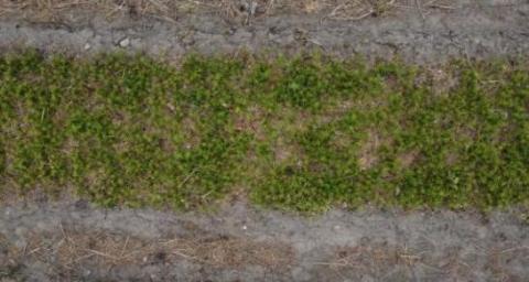
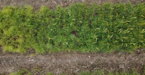
Figure 1. Dataset of Korean pines at different stages
2.2 Image processing module
All experimental processes were executed in a Linux environment, specifically under the Ubuntu18.04.5 operating system, accompanied by the cuDNN7.6.5 and Darknet framework, with Python 3.7 as the chosen programming language. The computational hardware consisted of a setup with 125.6 GB RAM, an Intel(R)Core(TM) i7-10750CPU @2.60GHz processor, and an NVIDIA RTX3060 VGA graphics card.
2.3 Image selection and processing
A collection of 298 drone-captured images, inclusive of POS data and control points from the selected research area, were imported into the Pix4D software where they were merged to form orthoimages. It was observed that under standard conditions, traditional Region of Interest (ROI) sampling methods failed to exploit the full potential of deep learning. Therefore, prior to any processing, it became imperative to categorically label the entire chosen sample area. As illustrated in Figure 1, Korean pines, contingent on their growth cycle stage, exhibit variations in color, dimension, and form when observed under natural lighting. Further characteristics of these pines are detailed, emphasizing the randomness in spike count and planting density.
The image resolution was documented to be 4000×2250 pixels, with the images being saved in jpg format. From the total dataset comprising 2000 drone-captured images, plant targets visible within the images were demarcated using rectangular boxes via the Labeling tool. Label data was stored in the PASCALVOC dataset format, capturing target type, coordinate position, width, and height, which were subsequently archived as xml files. For analytical purposes, the images were partitioned into a test dataset (500 images) and a training dataset (300 images).
3.1 Backbone network module
The YOLOv4 model contains many basic building blocks, and due to the large amount of convolution module computations, there are several feature maps, which increase the computational resources, leading to an increase in the model computation [8-10]. In the assembly of the feature pyramid, YOLOv4's primary feature extraction network, termed CSPDarknet53, channels three pivotal feature layers into the augmented feature extraction networks, specifically SPP and PANet [11, 12]. Given the extensive convolution calculations necessitated in this procedure, the operational speed is inherently compromised. To counteract this, GhostNet, which employs the Ghost module capable of generating analogous features with diminished parameters, was opted as a replacement for CSPDarknet53 in this research [12].
A delineation of GhostNet's architecture is provided in Table 1. This structure encompasses 11 sequences and spans across 21 network layers. Central to this design is the G-bneck, a residual module, with the Ghostmodule shaping the primary construct. It is discerned that the architecture of GhostNet predominantly consists of the G-bneck series [11]. From this configuration, three distinct effective feature layers were extracted: the inaugural effective feature layer (522×40), the secondary effective feature layer (262×112), and the tertiary effective feature layer (132×160). Upon the enhancement of this model, a notable reduction in its storage requirement was observed. Consequently, with GhostNet serving as the principal feature extraction network, a leaner model was realized, culminating in heightened detection efficiency.
Table 1. Architectural overview of GhostNet
|
Sequence |
Input |
Operation |
Output |
Step Size |
|
1 |
4162×3 |
Con2d 3×3 |
16 |
2 |
|
2 |
2082×16 |
GBN |
16 |
1 |
|
3 |
2082×16 |
GBN |
24 |
2 |
|
4 |
1042×24 |
GBN |
24 |
1 |
|
5 |
1042×24 |
GBN |
40 |
2 |
|
6 |
522×40 |
GBN |
40 |
1 |
|
7 |
522×40 |
GBN |
40 |
2 |
|
262×80 |
GBN×4 |
112 |
1 |
|
|
8 |
262×112 |
GBN |
112 |
1 |
|
9 |
262×112 |
GBN |
160 |
2 |
|
10 |
132×160 |
GBN×4 |
160 |
1 |
|
11 |
132×160 |
GBN |
|
|
3.2 The Dynamic Region-aware Convolution (DRConv) module
In the pursuit of accurately estimating seedling numbers through remote sensing image analysis and understanding the evolutionary trajectory of sown areas, an elevated precision in the detection model becomes imperative. Recognized for its capabilities, the DRConv is noted to automatically allocate filters, thereby enhancing detection precision. Concurrently, this mechanism is known to transpose channel filters into spatial dimensions, fortifying the representational capacity of convolution without incurring additional computational overhead.
For the objectives of this research, DRConv was integrated with GhostNet. Its inclusion was driven by two facets: necessity and superiority. On the necessity front, DRConv aptly satisfied the dual demands of amplifying seedling detection accuracy while judiciously managing computational expenditures. As for its superiority, not only did it bolster detection precision without compromising speed, but its inherent self-adaptive attributes, when synergized with GhostNet, showed a heightened adaptability specifically tailored for seedling detection within the realm of remote sensing imagery.
3.2.1 Overall structure
The structure of DRConv is given in Figure 2. Assuming: Z∈EI×C×V represents the input of standard convolution; I, T, and V respectively represent height, width, and channel; A∈RI×C represents spatial dimension, T∈RI×C×P represents output, Q∈RV represents standard convolution filter, * represents 2D convolution operation, then the feature mapping of the p-th output feature can be expressed as:
$T_{i, c, p}=\sum_{v=1}^v Z_{i, c, p} * Q_v^{(0)}(i, c) \in A$ (1)
In basic local convolution, assuming: Q∈RI×C×P represents filters that are not shared in spatial dimensions, Q(0)i,c,p represents a single non-sharing filter at the position of pixel (i,c) that is different from the standard convolution, then the following formula gives the expression of feature mapping of the p-th output feature:
$T_{i, c, p}=\sum_{v=1}^v Z_{i, c, p} * Q_{i, c, p}^{(0)}(i, c) \in A$ (2)
Based on above formula, the guided mask L={A0,...,Al-1} that can represent region division in spatial dimensions could be defined, wherein only one filer can be shared in each region, denoted as y∈ [0, l-1]. Let filter Qy∈RV correspond to region Ay, it can be assumed that the filter of the region is represented by L={Q0,...,Ql-1}, the v-th channel of Q(0)y is represented by Q(0)y,v, and any point in region Ay is denoted as (i, c), then the p-th channel of the output feature map of this layer can be written as:
$T_{i, c, h}=\sum_{v=1}^v Z_{i, c, v} * Q_{y, v}^{(0)}(i, c) \in A_y$ (3)
The implementation of DRConv has two main steps, including the setting of the learnable guided mask module and the filter generation module, and the functions of the two modules will be introduced in detail in the following text.
Figure 2. Structure of DRConv
3.2.2 The learnable guided mask module
Utilized within the architecture, the learnable guided mask module employs guided masks to segment spatial features into several distinct regions across spatial dimensions. This segmentation process has been observed to permit differentiated processing across these spatial regions, subsequently augmenting the model's adaptability and fortifying its competency in discerning intricate spatial configurations. Furthermore, it is through the guided mask that the filter distribution across spatial dimensions is determined. Filters are systematically allocated to their pertinent regions and are refined via the loss function. This procedural design enables filters to autonomously recalibrate their distribution in response to varying input spatial data, proving instrumental in the accurate capture of local image features and amplifying the model's proficiency in isolating and differentiating features within specific areas.
Specifically speaking, if a DRConv of size j×j contains l shared regions, then guided features with l channels could be constructed based on a standard convolution with a kernel size of j×j. Assuming: D∈RI×C×l represents guided feature, L∈RI×C represents guided mask, Di,c represents the guided feature vector at position (i,c), then for each position (i,c) in the spatial region, there is:
$L_{i, c}=\arg \max \left(\hat{D}_{i, c}^0, \hat{D}_{i, c}^1, \cdots, \hat{D}_{i, c}^{l-1}\right)$ (4)
For filters [Q0,...,Ql-1], QLi,c was generated by H(·), assuming Li,c represents the index describing the maximum channel size of guided feature D at position (i,c), then, the filter Q^i,c corresponding to position (i,c) can be attained:
$\hat{Q}_{i, c}=Q_{L_{i, c}}, L_{i, c} \in[0, l-1]=Q * L_{i, c}$ (5)
Through above operations, all positions established connections with filters, in the meantime, contextual similarity of pixels using the same filters reached the ideal state.
Then, a one-hot-form substitution D^ of the guided mask was introduced in the process of back propagation, then there is:
$\hat{D}_{i, c}^k=\frac{e^{D\,_{i, c}^k}}{\sum_{b=0}^{l-1} \,\,e^{D\,_{i, c}^b}} k \in[0, l-1]$ (6)
Through the processing of above formula, D^ki,c was made as close as possible to 0 or 1. Besides, Q^i,c can be regarded as a one-hot-form of filters [Q0,...,Q4l-1] multiplied by Li,c and can be approximated as [D^0i,c,...,D^l-1i,c], further, the gradient of D^ki,c can be attained based on the following formula:
$\nabla \hat{D}_{i, c}^k M=\nabla_{\hat{Q}_{i, c}}, \cdots, \hat{D}_{i, c}^{l-1} k \in[0, l-1]$ (7)
Assuming: < > represents the dot product, $\odot$ represents the element-by-element multiplication, ∇M represents the gradient of tensor with respect to the loss function, then the approximate back propagation is given by Eq. (5):
$\nabla D_{i, c} M=\hat{D}_{i, c} \Phi\left(\nabla_{\hat{D}_{i, c}} M-1\left\langle\hat{D}_{i, c}, \nabla_{\hat{D}_{i, c}} M\right\rangle\right)$ (8)
3.2.3 The filter generation module
The primary role of the filter generation module has been identified as the creation of tailored features, enabling the model to concentrate more accurately on distinct attributes of images. Such a design has been shown to augment both the detection precision and computational efficiency. Within each designated region, custom filters are produced by the filter generator to facilitate standard 2D convolution operations. Consequently, the model has been enabled to generate optimal filters tailored to the distinctive characteristics and demands of each specific region.
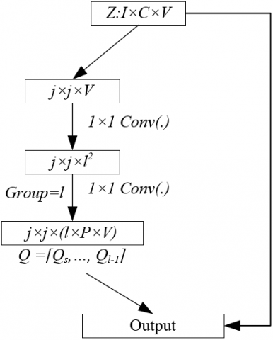
Figure 3 gives the structure of the filter generation module. Assuming: Z∈RI×C×V represents input, Q=[Q0,...,Ql-1] represents l filters, by setting the downsampling of sample Z as j × j, l filters could be generated, and the size of their kernels was all j × j. Next, two consecutive 1 × 1 convolutional layers employing sigmoid(·) as the activation function and without activation function were adopted. By generating custom features, the model can focus more precisely on the specific features of each image. This not only enhances the model’s adaptability to complex structures and different types of images, but also improves its detection precision.
Figure 3. Structure of the filter generation module
3.3 Model optimization for enhanced lightweight implementation
In contrast to traditional convolutional methods, DRConv has been recognized for its capability to efficiently extract feature information, maintaining computational complexity and translational properties unchanged. Enhanced convolutional representation in spatial dimensions is believed to augment DRConv's comprehension and feature capture capabilities within images. With smaller models exhibiting diminished representational prowess due to limited parameters, DRConv has been devised to augment spatial information capture without a surge in computational complexity. Consequently, an enhancement in the performance of smaller models was observed. Empirical results further substantiated the efficacy of DRConv for these models, highlighting a notable precision enhancement. Furthermore, the capability of DRConv to autonomously assign multiple filters to spatial regions exhibiting analogous representations has been recognized. Such a design is speculated to fortify the adaptability of smaller models to diverse spatial features, amplifying their efficacy with intricate structures and diverse image types.
Given the distinct growth phases of Korean pines observed in nursery gardens and the homogeneity of the target background within captured images, the integration of an attention mechanism within deep networks was found to significantly influence vital image information. Emphasis was placed more discerningly upon the seedlings, facilitating superior feature extraction. Although various attention mechanisms exist, such as the Squeeze-and-Excitation (SE) [13], it was discerned that SE predominantly contemplates the intrinsic channel data, overlooking the pivotal role of locational information [14]. Based on this observation, the Convolutional Block Attention Module (CBAM) was posited to exhibit superior performance [15].
Motivated by experimental insights, a fusion of DRConv with CBAM was suggested, aiming at precision enhancement. Such a combined approach is posited to considerably elevate detection precision without compromising on processing speed. CBAM, having gained traction for target detection tasks, represents a composite attention mechanism. It facilitates feature map interconnections across channels and space. However, the CAM and SAM calculations intrinsic to CBAM are believed to introduce substantial redundancies [6]. Thus, CBAM was incorporated within one of the two pivotal feature layers emanating from the backbone network, hypothesized to influence target features without inducing excessive redundancy. CBAM encompasses two distinct modules: the channel attention module and the spatial attention module, as elucidated in Figure 4.
Figure 4. The CBAM attention mechanism
Within this figure, 'Conv' is indicative of convolution, 'GAP' symbolizes global average pooling, and 'GMP' denotes global maximum pooling.
3.4 Optimization of the loss function
Optimizing the loss function is essential to the advancement of machine learning models, especially when precision and adaptability are imperative. The loss function's role in attenuating the Loss signal through adjusted weight values is established [16]. Such adjustments enable the provision of feedback when mispredictions occur and subsequently enhance the model's convergence speed. In recent studies, the GIoU loss function was employed as a metric for location regression loss assessment [17], while other researches [18, 19] incorporated the GIoU loss as the primary loss function.
For a nuanced capture of both spatial and temporal variations and growth characteristics inherent in seedlings, alongside the enhancement of the model's detection precision, convergence speed, and generalization capabilities, a distinctive approach was undertaken in this analysis. The evolution value of the seedling area over time, as determined by the Gaussian plume model, was utilized as the corrected value. Subsequently, a YOLOv4 confidence loss function was crafted. Recognizing the disparate morphological and distributional nuances seedlings manifest across growth stages, the employment of the Gaussian plume model's evolution value for loss function correction was hypothesized to bolster the model's adaptability to varied seedling growth phases and ambient conditions.
Leveraging the Gaussian plume model, the density V(z,t,x,y) of the Korean pine forest within the nursery garden at any given temporal instance can be represented as:
$V(z, t, x, y)=S(z) r^{-s\left[z-i\left(y-y_u\right)\right]\,^2} r^{-n t^2} r^{-v G^2}$ (9)
The variance equations are:
$\left\{\begin{array}{l}\delta_z^2=\frac{\int_0^{\infty}\left[z-i\left(y-y_u\right)\right]\,^2 V d z d y}{\int_0^{\infty} V d z d y} \\ \delta_t^2=\frac{\int_0^{\infty} t^2 V d y}{\int_0^{\infty} V d y} \\ \delta_x^2=\frac{\int_0^{\infty} G^2 V d z}{\int_0^{\infty} V d z}\end{array}\right.$ (10)
Formula of the evolution source is:
$W=\int_{-\infty}^{\infty} \int_{-\infty}^{\infty} i V d z d t d x d y$ (11)
Under the condition that the influence of time is not considered, constant terms s, n, and v can be calculated by the following equations:
$V\left\{\begin{array}{l}s=\frac{1}{2 \delta_z^2} \\ n=\frac{1}{2 \delta_t^2} \\ v=\frac{1}{2 \delta_x^2}\end{array}\right.$ (12)
By combining Eq. (9) with Eq. (11) and Eq. (12), the calculation formula of S(z) can be attained:
$S(z)=\frac{W}{2 \pi i \delta_z \delta_t \delta_x}$ (13)
Assuming: under an evolution source, z represents precipitation, t represents the supply amount of wastes, x represents sunlight intensity, y represents sunlight duration, then the density of seedlings can be written as V(z,t,x,y); S(z) represents the transition function, G represents the growth rate of seedlings; $\delta_z$, $\delta_y$, $\delta_x$ are evolution parameters in different directions; i represents the wind speed in the environment; W represents the degree of human intervention, then by combining Eq. (9) with Eq. (12) and Eq. (13), there is:
$V(z, t, x, y)=\frac{W}{(2 \pi)^{\frac{3}{2}} i \delta_z \delta_t \delta_x} \,\,e^{-\frac{\left[z-i\left(y-y_u\right)\right]\,^2}{2 \delta_z^2}} \,\,e^{-\frac{t^2}{2 \delta_t^2}} \,\,e^{-\frac{G\,^2}{2 \delta_x^2}}$ (14)
The modelling process in this paper only considered the evolution of seedling area over time, then the above formula can be simplified to:
$V(y)=\frac{W}{2 \pi i \delta_z \delta_t \delta_x} e^{-\frac{\left[i\left(y-y_u\right)\right]\,^2}{2 \delta_z^2}}$ (15)
From the analyzed video capturing the evolution of the seedling area, it was observed that the sown area for seedling targets rapidly attained a peak value, underscoring the significance of "primary seedling targets" within a specified temporal frame. For simulating the evolution trajectory of the seedling area, the Gaussian plume model was employed. Within the stipulated interval [1, 2], a corrected value was generated by the Gaussian function, reflecting the seedling area's temporal progression. This derived value was instrumental in amplifying the confidence score of prediction boxes encompassing targets identified proximate to the peak time. In essence, if targets were detected around or at the zenith of primary seedling target incidence, a bolstered confidence score was ascribed. Continuous iterative training ensured heightened model sensitivity towards the delineated "primary seedling targets". The integration of this corrected value fostered model refinement in a specific trajectory, culminating in a refined model adept at pinpointing primary seedling targets with augmented precision and confidence during real-time detection.
The confidence degree loss function is articulated as follows:
$\begin{aligned} & C O D_{L O(O B)} =\left\{\sum_{u=0}^{J \times J} \sum_{k=0}^L U_{u k}^{p n k}\left[V_u \log \left(\hat{V}_m\right)+\left(1-V_u\right) \log \left(1-\hat{V}_m\right)\right]\right\} * V \\ & +\sum_{u=0}^{J \times J} \sum_{k=0}^L U_{u k}^{N O}\left[V u \log \left(\hat{V}_m\right)+\left(1-V_u\right) \log \left(1-\hat{V}_m\right)\right]\end{aligned}$ (16)
Given the presence of numerous targets within the images, specific parameters were meticulously set to enhance the model's stability. A momentum factor of 0.963 was established, accompanied by an attenuation coefficient of 0.0005. The learning rate was initially fixed at 0.001, and the maximum iterations were capped at 400. Every set of 100 iterations resulted in the preservation of a weight file, culminating in a total of five distinct models.
Figure 5. Graphical representation of loss trends
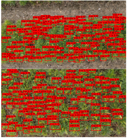
Figure 6. Actual detection image samples
It was discerned that model quality wasn't solely contingent on iteration numbers. Concerns arose regarding potential over-fitting stemming from redundant iterative training. Following the conclusion of training, these models underwent rigorous evaluations to discern the optimal model. Utilizing the dataset, the model's loss function underwent training, with pertinent alterations depicted in Figure 5. As evidenced from Figure 5, post the 200th iteration epoch, a stable convergence of the loss value was witnessed, accompanied by minute fluctuations. Figure 6 offers a visual representation of genuine detection images.
Figure 7 delineates the findings from the ablation experiments of DRConv, focusing on CSPDarknet53 and GhostNet in comparison to standard architectures across varied model size scales. A palpable observation from this figure is the superior performance of the DRConv-integrated version in comparison to the standard CSPDarknet53 across all scales. Most notably, smaller models witnessed the most pronounced precision enhancement, exemplified by the rise from 53 to 61.9. In contrast, larger models saw a more subdued precision increment. This aligns with prior assertions suggesting DRConv's capability to efficiently distill features sans computational complexity augmentation, especially accentuated in smaller models. A similar trend was observed in the DRConv-GhostNet variant, which consistently overshadowed the performance of the standard GhostNet across all scales. The enhancement in precision, especially in smaller models (e.g., 0.5 scale), was marked, elevating from 60.8 to 67. This reinforced the notion that DRConv bolstered semantic expression capacity within spatial dimensions, with smaller models, characterized by weaker expression abilities, reaping pronounced benefits.
Upon juxtaposition of the two DRConv variations with distinct architectures, it was observed that DRConv-GhostNet typically displayed marginally superior performance compared to DRConv-CSPDarknet53 at identical model scales. This disparity can be attributed to the intrinsic structure and nuances of GhostNet, suggesting a synergistic effect when DRConv is amalgamated with specific backbone networks.
As demonstrated in Figure 8, the precision of the model at various iteration stages is graphically represented. Within the initial training phases, the model's precision was observed to commence at a notably low tier. However, as training progressed, an elevation to higher precision levels was noted. The trajectory of precision enhancement was not consistently linear; intermittent fluctuations were evident, suggesting potential amendments to learning rates, regularization, or other hyperparameters might be beneficial for achieving a more consistent training phase. During the latter stages of the iterative process, the precision's rate of growth decelerated, plateauing at an elevated threshold. This behavior suggests that the model could be nearing its maximum potential. While the precision results indicate a predominantly successful training regime and an elevated performance tier, further optimization and detailed analysis remain imperative.
The model's recall, in contrast, began at elevated levels during the early training stages. This recall rate consistently exhibited an upward trajectory as training continued. Although the ascent in recall rate was predominantly linear, minor fluctuations in its midpoint warrant further scrutiny. The underlying cause of these deviations — whether attributable to the dataset, a necessity for hyperparameter modification, or an indication of requisite structural model adjustments — remains a topic for further exploration. By the culmination of the training period, the recall rate exhibited a state of stabilization, suggesting the model had successfully assimilated the pivotal features, reflecting high performance. Despite this apparent efficacy, subtle optimizations might further elevate the model to its apex.
Figure 9. P-R curve analysis of the constructed model
Figure 9 depicts the Precision-Recall (P-R) curve, a renowned metric for gauging model performance across varying thresholds. A careful examination of Figure 9 permits an analytical interpretation of the precision's trend relative to recall. At suboptimal recall levels, an exceedingly high precision was documented, indicative of superior classification efficacy during this phase. However, with an augmented recall rate, a concomitant decline in precision was observed. This behavior suggests a conscious trade-off: a sacrifice in precision to encapsulate an increased volume of positive samples. As recall rates verged on their maximum, a precipitous decline in precision was noted, highlighting potential model vulnerabilities necessitating further analysis and adjustment.
Utilizing a consistent dataset and identical parameters, performance indicators for the proposed model were juxtaposed against three benchmarks: the YOLOv4 model, the Faster R-CNN model [20], and the SSD model [21]. These comparative results are catalogued in Table 2.
From the data presented in Table 2, it is discerned that the proposed model achieved the apex in precision, registering at 91.85%. Comparative analyses revealed that precision rates for the other models hovered in proximity, with YOLOv4 at 89.78%, SSD at 89.25%, and Faster R-CNN at 88.86%. Additionally, the highest recall rate was attributed to the proposed model at 89.47%. In contrast, the YOLOv4's recall rate was documented at 85.12%, with the subsequent models registering even lower values. These findings underscore the proposed model's superior performance concerning recall.
Regarding the Average Precision (AP) value, the proposed model again demonstrated a marginal supremacy with a value of 90.05%. Both YOLOv4 and SSD manifested closely aligned AP values, 88.56% and 88.46% respectively, while the Faster R-CNN trailed with 87.35%.
The F1 score, a metric harmonizing precision and recall, proffers insights into the model's holistic performance. In this domain, the proposed model was observed to surpass its counterparts, achieving a score of 90.64%. The other models consistently recorded F1 scores below the 90% threshold.
In terms of computational efficiency, the proposed model was distinguished by its swiftness, necessitating a mere 28 ms for detection. This speed contrasts starkly with other models, most notably the Faster R-CNN, which demanded a significantly elongated time of 45 ms.
This analysis elucidates that the proposed model transcends YOLOv4, Faster R-CNN, and SSD across an array of pivotal performance indicators, encompassing precision, recall, average precision, F1 score, and per-image detection time. Such superior performance is inextricably linked to the intricate model design and optimization expounded upon in preceding sections. This includes, but is not limited to, components like the YOLOv4 confidence loss function, which was formulated based on values rectified by the Gaussian plume model.
Table 2. Comparative analysis of model performance
|
Model |
Precision /% |
Recall Rate /% |
AP / % |
F1 |
Detection Time per Image |
|
The proposed model |
91.85 |
89.47 |
90.05 |
90.64 |
28ms |
|
YOLOv4 |
89.78 |
85.12 |
88.56 |
87.38 |
30ms |
|
Faster R-CNN |
88.86 |
84.78 |
87.35 |
86.77 |
45ms |
|
SSD |
89.25 |
84.86 |
88.46 |
86.99 |
31ms |
In the present investigation, the enumeration of Korean pine seedlings was meticulously performed using a refined YOLOv4 model. Rapid identification of seedling targets was achieved, and their count was determined with precision. An impressive recall rate of 88.47 was observed for the model, underscoring its superiority compared to other prevalent target detection models. Within the scope of the experimentation, only test set images were subjected to predictions, and the dimensions of the predicted images remained congruent with the input dimensions. Comprehensive analysis involving the entirety of the sample set was not executed; therefore, ensuing studies are anticipated to delve into large-scale and high-resolution plant enumeration methodologies, potentially incorporating strategies like cropping, predictive analysis, and splicing of expansive regions.
This paper was supported by National Natural Science Foundation (Grant No.: 31970454).
[1] Li, S. (2014). On the sixth in formation revolution. China New Telecommunications, 16(14): 3-6. https://doi.org/10.3969/j.issn.1673-4866.2014.14.002
[2] Cao, L., Zhou, K., Shen, X., Yang, X., Cao, F., Wang, G. (2022). The statues and prospects of smart forestry. Journal of Nanjing Forestry University (Natural Science Edition), 46(6): 83-95. https://doi.org/10.12302/j.issn.1000-2006.202209052
[3] Wang, X.S., Huang, X.Y., Fu, H. (2010). Study surveys on tree image extraction in a complex background. Journal of Beijing Forestry University, 32(3): 197-203.
[4] Qi, J. (2018). Spruce statistics software development based on HOG feature cascade classifier. Master's thesis, Beijing Forestry University, China.
[5] Zhang, Z.W., Zhao, P., Han, J.C. (2021). Research on measurement method of single tree height using binocular vision. Journal of Forestry Engineering, 6(6): 156-164. https://doi.org/10.13360/j.issn.2096-1359.202012009
[6] Yuan, X.P., Wang, Z., Han, J., Chen, Y. (2023). Improved YOLOv4 target detection method for complex traffic scenes. Science Technology and Engineering, 23(6): 2509-2517. https://doi.org/10.12404/j.issn.1671-1815.2023.23.06.02509
[7] Chen, Y.L., Zhang, X.J., Chen, X.J. (2022). Identification of navel orange trees based on deep learning algorithm YOLOv4. Science of Surveying and Mapping, 47(2): 135-144, 191. https://doi.org/10.16251/j.cnki.1009-2307.2022.02.018
[8] Bochkovskiy, A., Wang, C.Y., Liao, H.Y.M. (2020). Yolov4: Optimal speed and accuracy of object detection. arXiv preprint arXiv:2004.10934.
[9] Wang, C.Y., Liao, H.Y.M., Wu, Y.H., Chen, P.Y., Hsieh, J.W., Yeh, I.H. (2020). CSPNet: A new backbone that can enhance learning capability of CNN. In 2020 IEEE/CVF Conference on Computer Vision and Pattern Recognition Workshops (CVPRW), Seattle, WA, USA, pp. 390-391. https://doi.org/10.1109/CVPRW50498.2020.00203
[10] Liang, X.T., Pang, Q., Yang, Y., Wen, C.W., Li, Y.L., Huang, W.Q., Zhang, C., Zhao, C.J. (2022). Online detection of tomato defects based on YOLOv4 model pruning. Transactions of the Chinese Society of Agricultural Engineering (Transactions of the CSAE), 38(6): 283-292. https://doi.org/10.11975/j.issn.1002-6819.2022.06.032
[11] Min, K., Lee, G.H., Lee, S.W. (2022). Attentional feature pyramid network for small object detection. Neural Networks, 155: 439-450. https://doi.org/10.1016/j.neunet.2022.08.029
[12] Zhang, R.H., Ou, J.S., Li, X.M., Ling, X., Zhu, Z., Hou, B.F. (2023). Lightweight algorithm for pineapple plant center detection based on improved an YoloV4 model. Transactions of the Chinese Society of Agricultural Engineering (Transactions of the CSAE), 39(4): 135-143. https://doi.org/10.11975/j.issn.1002-6819.202210133
[13] Hu, J., Shen, L., Albanie, S., Sun, G., Wu, E. (2019). Squeeze-and-Excitation Networks. IEEE Transactions on Pattern Analysis and Machine Intelligence, 42(8): 2011-2023. https://doi.org/10.1109/TPAMI.2019.2913372
[14] Che, X.J., Chen, H.Y. (2022). Muti⁃Object dishes detection algorithm based on improved YOLOv4. Journal of Jilin University (Engineering and Technology Edition), 52(11): 2662-2668. https://doi.org/10.13229/j.cnki.jdxbgxb20211013
[15] Woo, S., Park, J., Lee, J.Y., Kweon, I.S. (2018). CBAM: Convolutional block attention module. In Proceedings of the European Conference on Computer Vision (ECCV), Munich, Germany, pp. 3-19. https://doi.org/10.1007/978-3-030-01234-2_1
[16] Yu, J., Jiang, Y., Wang, Z., Cao, Z., Huang, T. (2016). Unitbox: An advanced object detection network. In Proceedings of the 24th ACM International Conference on Multimedia, Amsterdam, The Netherlands, pp. 516-520. https://doi.org/10.1145/2964284.2967274
[17] Rezatofighi, H., Tsoi, N., Gwak, J., Sadeghian, A., Reid, I., Savarese, S. (2019). Generalized intersection over union: A metric and a loss for bounding box regression. In Proceedings of the IEEE/CVF Conference on Computer Vision and Pattern Recognition (CVPR), Beach, CA, USA, pp. 658-666. https://doi.org/10.1109/CVPR.2019.00075
[18] Zheng, Z., Wang, P., Liu, W., Li, J., Ye, R., Ren, D. (2020). Distance-IoU loss: Faster and better learning for bounding box regression. Proceedings of the AAAI Conference on Artificial Intelligence, 34(7): 12993-13000. https://doi.org/10.1609/aaai.v34i07.6999
[19] Chen, X.S., Wu, C.P., Dang, P.N., Liang, J., Liu, S.J., Wu, T. (2023). Improved lightweight YOLOv4 model-based method for the identification of shrimp flesh and shell. Transactions of the Chinese Society of Agricultural Engineering (Transactions of the CSAE), 39(9): 278-286. https://doi.org/10.11975/j.issn.1002-6819.202303076
[20] Ren, S., He, K., Girshick, R., Sun, J. (2016). Faster R-CNN: Towards real-time object detection with region proposal networks. IEEE Transactions on Pattern Analysis and Machine Intelligence, 39(6): 1137-1149. https://doi.org/10.1109/TPAMI.2016.2577031
[21] Liu, W., Anguelov, D., Erhan, D., Szegedy, C., Reed, S., Fu, C.Y., Berg, A.C. (2016). SSD: Single shot multibox detector. In 14th European Conference, Amsterdam, The Netherlands, pp. 21-37. https://doi.org/10.1007/978-3-319-46448-0_2