Rajamanickam Thamizhamuthu*![]() | Subramanian Pitchiah Maniraj
| Subramanian Pitchiah Maniraj![]()
© 2023 IIETA. This article is published by IIETA and is licensed under the CC BY 4.0 license (http://creativecommons.org/licenses/by/4.0/).
OPEN ACCESS
This paper introduces a sophisticated dermoscopic image classification system (DICS) leveraging deep learning techniques for accurate skin lesion classification. The DICS comprises four distinct modules: i) Skin Lesion Segmentation (SLS), ii) Feature Extraction (FE), iii) Feature Selection (FS), and iv) Image Classification (IC). The SLS module preprocesses the input dermoscopic image and employs a color k-means clustering approach for segmentation. Subsequently, in the FE module, three types of features are extracted, including 4th order Color Moments (CM), a statistical model based on Generalized Autoregressive Conditional Heteroscedasticity (GARCH), and texture features derived from Local Binary Patterns (LBP). The predominant features are then selected in the FS module using a statistical t-test. Finally, the IC module classifies dermoscopic images as normal or melanoma using a deep learning approach. The DICS demonstrates promising results, achieving 99% and 100% accuracy in normal/abnormal and benign/malignant classifications, respectively, when tested on the PH2 database. This robust classification system has the potential to contribute significantly to the field of dermatological image analysis.
image classification system, deep learning, feature extraction, colour moments, local binary pattern, statistical model
Skin cancer, characterized by the uncontrolled growth of skin cells, is a growing global concern marked by increasing incidence and mortality rates. In 2018, the United States reported an estimated 91,270 new melanoma cases and 9,320 deaths [1]. Worldwide, over 232,000 new melanoma cases and approximately 55,000 deaths were estimated in 2012, with men exhibiting a higher mortality rate than women. Early diagnosis and treatment of melanoma are crucial, as it can spread rapidly throughout the body. Consequently, numerous Computer-Aided Diagnosis (CAD) systems have been developed in recent years to screen and detect cancers.
A non-invasive method for skin lesion classification with real-time alerts for skin burns is presented in the study [2], utilizing texture, color, and shape features for early lesion classification via a Support Vector Machine (SVM) classifier. In the study [3], a Multi-Layer Perceptron (MLP) network is trained on color and edge characteristics of lesions for dermoscopic image classification systems (DICS), employing the backpropagation algorithm for effective lesion classification.
Melanoma diagnosis using wavelet-based features is explored in the study [4], where wavelet-based features are integrated with geometrical and border-based features. Four classifiers, including SVM, random forest, naive Bayes, and logistic tree model, are employed. In the study [5], a fixed grid wavelet network is utilized for melanoma diagnosis, with the relief algorithm selecting ten features from color, shape, and texture for adequate classification.
An approach for skin lesion segmentation and classification using a convolutional neural network is discussed in the study [6]. A fully convolutional residual network is employed for segmentation, while a deep residual network is used for classification, avoiding degradation problems through residual learning. In the study [7], a symbolic regression algorithm-based skin lesion classification is described, using clinically significant colors to compute malignancy scores and applying a k-means clustering approach to reduce the number of colors in dermoscopic images.
A melanoma classification method based on pigment network features, along with color, texture, and shape features, is presented in the study [8]. Ordinal regression and logistic regression learning algorithms are employed for classification. In the study [9], a neural network ensemble model for dermoscopic image classification is described. Initially, a self-generating neural network segments the skin lesion, followed by the extraction of color, shape, and texture feature descriptors. A network ensemble model combining backpropagation and fuzzy-based networks is used for classification.
A decision support system for melanoma diagnosis is discussed in the study [10], which investigates pigmented skin lesions. Following segmentation, texture, color, asymmetry, and border features are extracted, and a Bayesian network is used for classification. The final decision incorporates patient-related data such as age, gender, skin type, and body part. In the study [11], multispectral image analysis for melanoma classification is explored, using the mean energy of Daubechies-3 wavelet decomposed images as features and fuzzy membership functions for classification.
The primary objective of this study is to determine skin lesion abnormality severity with maximum accuracy. Previous studies have predominantly utilized color, shape, and texture features of skin lesions. Advanced modeling techniques can be applied to skin lesions, allowing model parameters to serve as features and enabling dimensionality reduction. The recent introduction of the Generalized Autoregressive Conditional Heteroscedasticity (GARCH) model in various signal processing applications has yielded improved performance. Consequently, this study analyzes the parameters of the GARCH model and standard features, such as color and texture, for DICS. Dominant features are selected using a statistical test and applied to deep learning for determining skin lesion abnormality. This paper presents an efficient CAD system for skin cancer diagnosis using dermoscopic images. Section 2 details the methods and materials employed by DICS, followed by a discussion of the experimental results in Section 3. The conclusion of this study is presented in the final section.
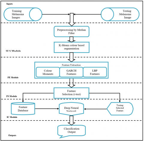
The DICS consists of the following modules: SLS, FE, FS, and IC modules. The following subsections explain these modules clearly and in detail. The idea of robust DICS is illustrated in Figure 1.
Figure 1. Flow of DICS for the diagnosis of skin cancer
2.1 SLS module
This is the first module of DICS where the exact skin cancer region is segmented using a k-means clustering approach on RGB (Red, Green, and Blue) colour images. K-means clustering is primarily a color-based segmentation approach that uses the colour values of the pixels in the image to cluster them into different groups. This means that pixels with similar color values are grouped, which can help to isolate the skin cancer region from the rest of the image. It does not require prior knowledge or training data to segment the image, i.e., an unsupervised learning approach. The algorithm involves the initialization of the cluster centers and continues to iterate until a convergence criterion is met. The output of the k-means clustering algorithm is a set of clusters, where each cluster corresponds to a different color region in the image.
Before segmentation, the image is smoothed by an averaging filter in the colour domain with a predefined window size which will remove noise and hair in the dermoscopic images. A larger sliding window of size 21×21 reduces the intensity variation between pixels, so noises and hairs will be removed completely. Let us consider a dermoscopic image DI. The pixel value of DI is represented by DIij, for i, j=1, ..., n, where n is the size of the image. The output Oij from the linear filter of size (2m+1)×(2m+1) is denoted by.
$O_{i j}=\sum_{x=-m}^m \sum_{y=-m}^m w_{x y} D I_{i+x, j+y}$ for $i, j=(m+1), . .(n-m)$ (1)
where, wxy for x, y=-m, ..., m is the weight of the filter. In this study, a linear filter (average filter) of size 21×21 (m=10) is used to smooth the image; hence, the weight is assigned equally to 1/21 for wxy. The application of this filter to DI replaces each pixel with the average of pixels values in a 21×21 window centered on that pixel. For simplicity, let us consider a 3×3 filter. The averaging is carried out over this window size is defined by:
$\begin{aligned} O_{i j}= & \left(w_{-1,-1} D I_{i-1, j-1}+w_{-1,0} D I_{i-1, j}+w_{-1,1} D I_{i-1, j+1}+\right. \\ & w_{0,-1} D I_{i, j-1}+w_{0,0} D I_{i, j}+w_{0,1} D I_{i, j+1}+ \\ & \left.w_{1,-1} D I_{i+1, j-1}+w_{1,0} D I_{i+1, j}+w_{1,1} D I_{i+1, j+1}\right) / 9\end{aligned}$ (2)
Figure 2 shows the preprocessed dermoscopic images.
Figure 2. (a) Input dermoscopic images (Top Row images) (b) Smoothed images (Bottom row)
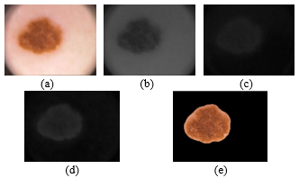
The RGB colour image is converted into L*a*b* colour space to quantify the visual differences. Figure 3 shows the filtered image's L,*a, and *b components. The conversion formula is as follows:
$L=11.6 h\left(\frac{Y}{Y_w}\right)-16$ (3)
$a=500\left[h\left(\frac{X}{X_w}\right)-h\left(\frac{Y}{Y_w}\right)\right]$ (4)
$b=200\left[h\left(\frac{Y}{Y_w}\right)-h\left(\frac{Z}{Z_w}\right)\right]$ (5)
where, $h(q)=\left\{\begin{array}{ll}q^{\frac{1}{3}} & q>0.008856 \\ 7.7879 q+\frac{16}{116} & q \leq 0.008856\end{array}\right\}$ .L, a, and b represent the lightness of the colour, red minus green and green minus blue. Also, X, Y, and Z correspond to R, G, and B channels, Xw, Yw, and Zw are reference white tri-stimulus values. This conversion enables obtaining all colour information in only two channels; a* and b*. Hence, k-means clustering is easily applied to cluster the colour information. It partitions the given data into k clusters. As the dermoscopic images contain skin lesions (abnormal region), unaffected skin region (normal skin area), and some background information (parts other than skin), the k value is set to 3. The steps to compute k-means clustering (k=3) for skin lesion segmentation are given below:
1. Randomly choose three initial clusters $\left(m_1^{(1)}, m_2^{(1)}\right.$ and $\left.m_3^{(1)}\right)$. The superscript identifies the initial cluster number.
2. The k-means clustering proceeds with assignment and update steps. These steps are iterated until it converges in the update step when the assignment no longer changes.
(a) Assignment step: In this step, each observation (zp) is assigned to one of the clusters (C), which has the least squared Euclidean distance. Thus, each observation (zp) is assigned to exactly one cluster $\left(C^{(t)}\right)$. It is defined by:
$C_i^{(t)}=\left\{z_p:\left\|z_p-m_i^{(t)}\right\|^2 \leq\left\|z_p-m_j^{(t)}\right\|^2 \forall j, 1 \leq j \leq 3\right\}$ (6)
(b) Update step: This step updates the means of the observations (z) in the new clusters ( $C_i^{(t)}$ ).
$m_i^{(t+1)}=\frac{1}{\left|C_i^{(t)}\right|} \sum_{z_j \in C_i^{(t)}} z_j$ (7)
Figure 3. RGB to L*a*b Conversion (a) RGB image (b) L channel (c) *a channel (d) *b channel (e) segmented lesion
The k-means clustering algorithm is widely applied in many medical image processing applications using gray-scale images. More information about the k-means clustering algorithm can be obtained from [12]. This study is applied to colour images with the help of colour information in a* and b* channels. Figure 3 (d) shows the segmented lesion.
The colour information in a* and b* channels are combined and fed to the k-means clustering to segment the lesion effectively. The obtained cluster (segmented area) from the k-means approach is superimposed with the preprocessed image to get the original skin lesion, shown in Figure 3(d).
2.2 FE module
Three different types of features, such as CM of up to 4th order, GARCH, and texture features by LBP, are discussed in the following sub-sections.
2.2.1 Colour moments
As the colour of the skin lesion plays an essential role in dermoscopic image classification, CMs are an excellent feature to use. They are computed from the RGB colour model, which characterizes the colour distribution in the skin lesion regions. Table 1 shows the CMs used in DICS. The total number of colour features extracted in this phase is 12.
Table 1. Colour moments
|
Colour Moments |
Formula |
Description |
|
1st order |
$\bar{\mu}=\frac{1}{H W} \sum_{i=1}^H \sum_{j=1}^W I(i, j)$ |
Average colour |
|
2nd order |
$\sigma=\frac{1}{H W} \sum_{i=1}^H \sum_{j=1}^W(I(i, j)-\bar{\mu})^2$ |
dispersion |
|
3rd order |
$\gamma=\frac{1}{H W} \sum_{i=1}^H \sum_{j=1}^W\left(\frac{I(i, j)-\bar{\mu}}{\sigma}\right)^3$ |
Shape of colour distribution |
|
4th order |
$k=\frac{1}{H W} \sum_{i=1}^H \sum_{j=1}^W\left(\frac{I(i, j)-\bar{\mu}}{\sigma}\right)^4-3$ |
Shape of colour distribution |
|
where, I is the segmented image, and H and W are the height and width. |
||
2.2.2 GARCH features
The GARCH model was developed by Bollerslev [13]. As the name implies, GARCH includes a feedback mechanism to predict future variances using past variances. The robustness of a GARCH model depends on several factors, including the quality and quantity of data used to estimate the model parameters and the choice of model specification. It requires sufficient high-quality data to accurately estimate the model parameters. The proposed system uses high-quality dermoscopic images from the PH2 database. It is also essential to carefully consider the assumptions and limitations of model specification and the best fits the data are chosen. The GARCH model has been applied to speech processing [14, 15], image de-noising [16], and signal classification [17]. If the intensity information in each colour channel is modeled with GARCH, then the parameters of GARCH can be used as features. The GARCH (p,q) process is defined by:
$\varepsilon_t=\sigma_t z_t$ (8)
where, σt is the conditional standard deviation and zt is a random variable drawn from a Gaussian distribution with zero mean and unit variance. Also, σt is a process such that:
$\begin{aligned} & \sigma_t^2=\alpha_0+\sum_{i=1}^q \alpha_i \varepsilon_{t-i}^2+\sum_{j=1}^p \beta_j \sigma_{t-j}^2 \\ & \text { where } q>0 ; p \geq 0 ; \alpha_0>0 ; \alpha_i \geq 0 ; \beta_j \geq 0 ; 1 \leq i \leq q ; \\ & 1 \leq j \leq p ; \text { and } \sum_{i=1}^q \alpha_i+\sum_{j=1}^p \beta_j<1\end{aligned}$ (9)
In this study, the parameters of the GARCH model with units p(1) and q(1) are used. That is, GARCH(1,1):
$\sigma_t^2=\alpha_0+\alpha_1 \varepsilon_{t-1}^2+\beta_1 \sigma_{t-1}^2$ (10)
The constant parameter in Eq. (10) such as α0, α1and β1 can be obtained using maximum likelihood estimation [17]. These parameters, along with the conditional mean constant, are considered features. To fit the GARCH model, the condition means are assumed to be constant for simplicity as GARCH processes are independent of conditional mean on the past, and it depends only on the conditional variance on the past. The total number of GARCH features extracted in this phase is 12.
2.2.3 LBP features
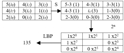
LBP is an efficient local descriptor in many pattern recognition approaches [18, 19]. It is invariant against any intensity changes due to illumination variances. It uses simple thresholding of neighboring pixels inside a 3x3 window with a threshold value equal to the intensity of the centre pixel. LBP features are computed by using the following Eq. (11):
$L B P\left(X_c, Y_c\right)=\sum_{n=0}^7 2^n S\left(i_n-i_c\right)$ (11)
where, (Xc, Yc) is the centre pixel of a 3x3 window, S is the threshold function ic and in represents the value of the central pixel and the value of nth neighborhood pixels, respectively. The threshold function S is defined by:
$S= \begin{cases}0 & \text { if } i_n-i_c<0 \\ 1 & \text { if } i_n-i_c \geq 0\end{cases}$ (12)
Figure 4. LBP Process
The application of Eq. (11) the whole image produces LBP with 256 different patterns. All these patterns are extracted for each colour channel without considering the border. The total number of LBP features extracted in this phase is 768. Figure 4 shows the working process of LBP. The value inside the parenthesis is obtained by Eq. (12).
2.3 FS module
The DICS extracts the features such as CM of up to 4th order, parameters of the GARCH model, and texture features by LBP to classify skin lesions. The feature dimension is 792 per dermoscopic image. The extracted features by the above steps from 2.2.1 to 2.2.3 may contain redundant information, which may degrade the system's performance. To overcome this, the FS module is introduced in the DICS. A commonly used hypothesis test, the t-test, is used to decide whether the extracted features are significantly different from each other or not. The features are ranked by class separability criteria to identify the dominant feature set.
Let us consider, N={Nk1, Nk2, ..., Nkf 1≤k≤n1} be the extracted features from n1 several normal training samples and A={Ak1, Ak2, ..., Akf 1≤k≤n2} the extracted features from n2 several abnormal training samples. Each normal and abnormal case consists of f number of features. Let the means of each feature in groups N and A are defined by:
$m_{N_i}=\frac{1}{n_1} \sum_{k=1}^{n_1} N_{k i} \quad 1 \leq i \leq f$ (13)
$m_{A_i}=\frac{1}{n_2} \sum_{k=1}^{n_2} A_{k i} 1 \leq i \leq f$ (14)
The t-test statistic value is given by:
$t_i=\frac{m_{N_i}-m_{A_i}}{\sqrt{\frac{V^2}{n_1}+\frac{V^2}{n_2}}} \quad 1 \leq i \leq f$ (15)
where, $V^2=\frac{\sum_{x=1}^{n_1}\left(N_{x i}-m_{N_i}\right)^2+\sum_{y=1}^{n_2}\left(A_{y i}-m_{A i}\right)^2}{n_1+n_2-2}$.
It is observed from Eq. (15), that the t-test provides f number of t values. The feature with a high t-value indicates that the two classes (normal and abnormal) are significantly different. In this stage, only the dominant elements are selected by t-test, and the classification is done in the next step by the selected features as Dominant Features (DF) in a predefined percentage (1%, 2%, and 3%) of total feature dimension.
2.4 IC module
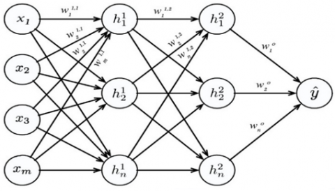
This module employs a deep learning approach for dermoscopic image classification. Deep learning adds more hidden layers between input and output layers to nonlinear model relationships, whereas traditional neural networks normally have one hidden layer [20]. A simple deep-learning architecture with two hidden layers is shown in Figure 5.
Let us consider X=[x1, x2, ..., xm] be the input feature vector with m features that forms the input layer of the neural network. The ith neuron in the jth hidden layer is denoted by, $h_i^j$ and the corresponding weight is denoted by $w_k^{i, j} \quad 1 \leq k \leq m$. The output of the first hidden neuron in the first hidden layer, i.e., $h_1^1$ is obtained by the dot product of features in the input feature vector X with their corresponding weight. It is defined by:
$z=\sum_{i=1}^m w_i^{1,1} x_i+$ bias (16)
The obtained dot product of $h_1^1$ is fed into an activation function $h_1^1=f(z)$ to get the neuron's output. This procedure is repeated for all neurons in each hidden layer. As the step function has no useful derivatives, the tansig function is used in this study as an activation function and works better for backpropagation. The backpropagation is a descent algorithm that minimizes the error at each iteration when the error signal is backpropagated to the lower layer. The weights in this network are adjusted, so that error rate reduction usually occurs in a decent direction.
Figure 5. Neural network architecture with two hidden layers
Figure 6. Tan-Sigmoid function in the classifier input layer
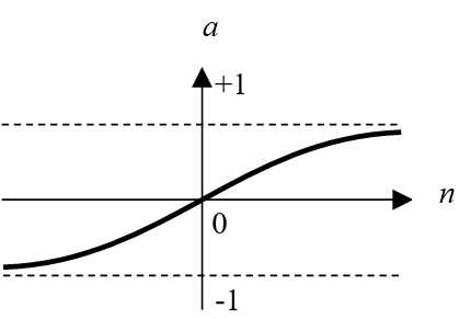
The training is usually done based on the error signal with an iterative updating of the weights, which uses the mean-squared error function of the negative gradients. The error signal is the difference between the actual and the desired output values multiplied in the input layer by the sigmoid activation function $\left(a=\operatorname{tansig}(n)=\frac{2}{1+e^{-2 a}}-1\right)$.
The tansig function is a popular activation function mainly used in the hidden layers. It has several desirable properties. First, it is a smooth, continuous function that can be easily differentiated and used in gradient-based optimization algorithms. Second, a nonlinear function allows neural networks to model complex relationships between inputs and outputs. The choice of activation function, including the tansig function, depends on the nature of the data and the task at hand. The tansig function is a hyperbolic tangent function that maps its input to a range between -1 and 1. It accelerates the convergence of the backpropagation method and is well-suited for modeling nonlinear relationships between inputs of normal and abnormal dermoscopic images. Figure 6 shows the tansig function in the classifier input layer.
The classifier output is obtained from the results of jth the hidden layer. Since the classifier is trained to produce only one output, either normal or abnormal, the weight w0 consists of n weights with $w_1^o, w_2^o, \ldots w_n^o$. It is defined by:
$z=\sum_{i=1}^n w_i^o h_i^j+$ bias (17)
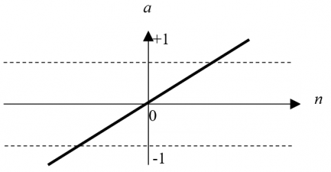
The obtained dot product is fed into an activation function $\hat{y}=f(z)$ to get the final classifier output. The function used in the output layer is the linear function (a=purelin(n)) which is shown in Figure 7. While training the classifier, the abnormal inputs are given with class labels as '1' and normal with class labels '0'. Thus, for a testing sample, if the classifier output is greater than 0, the testing sample is classified as abnormal else it is classified as normal.
Figure 7. Linear function in the classifier output layer
After the FS module, the deep learning network is trained using the selected features with ten hidden layer structures and validated using a ten-fold cross-validation technique.
The DICS designed in section 2 is analyzed using the PH2 database [21, 22]. It contains 200 dermoscopiccolour images with melanocytic lesions. The resolution of these images is 768x560 pixels. There are 80 normal and 120 abnormal images available for classification. The classification scenario is a two-level deep learning approach. In the 1st level deep learning approach, the task is to classify the image as normal or abnormal. Then in the 2nd level deep learning approach, the abnormal severity is classified again into benign/malignant.
Once the features are extracted, they are analyzed for the classification of dermoscopic images individually. Then, the FS module is introduced to select DFs from the fused feature set. The k-fold cross-validation is employed, and the performance of DICS is computed using different features; CM, GARCH, LBP, DF (1%), DF (2%), and DF (3%). The definitions of various performance metrics used in DICS are shown in Table 2,
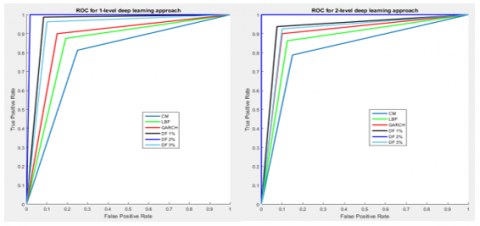
Table 2 defines T+ and T- as the number of correct classifications of abnormal and normal skin images, respectively. Similarly, F- and F+ are defined as the number of incorrect classifications of abnormal and normal skin images, respectively. Apart from these performance metrics, a graphical plot called Receiver Operating Characteristics (ROC) is drawn between Sen and 1-Spe. It shows the diagnostics ability of DICS by the area below the curve. Tables 3 and 4 show the performances of 1st- and 2nd-level deep learning approaches for the classification of skin cancer, respectively.
It is observed from Tables 3 and 4 that the number of correct classifications (T+ and T-) is more than others, which means that the DF (2%) has more promising results than other features used in DICS for skin cancer classification. The DICS achieves 98.33% and 100% sensitivity for 1st and 2nd stage deep learning approaches while using DF (2%) features. Also, it is noted that 100% specificity is achieved at both classification stages. Among the three features (CM, LBP, and GARCH), GARCH has the highest accuracy of 87% (1st stage) and 90% (2nd stage) than others. Figure 8 shows the ROCs of 1st and 2nd stage deep learning approaches.
Table 2. Performance matrices of DICS
|
Performance measure |
Description |
Formula |
|
Sensitivity (Sen) |
It refers to the ability of the DICS to detect abnormal cases correctly. |
$\operatorname{Sen}=\frac{T+}{(T+)+(F-)}$ |
|
Specificity (Spe) |
It refers to the ability of DICS to detect normal cases correctly. |
$S p e=\frac{T-}{(T-)+(F+)}$ |
|
Accuracy (Acc) |
It refers to the overall accuracy of DICS. |
$A c c=\frac{(T+)+(T-)}{(T+)+(F-)+(T-)+(F+)}$ |
|
T+ →True Positive, F- →False Negative, T- →True Negative and F+ →False Positive |
||
Table 3. Performance of 1st level deep learning approach
|
Metrics |
Features |
|||||
|
CM |
LBP |
GARCH |
DF (1%) |
DF (2%) |
DF (3%) |
|
|
T+ |
90 |
97 |
102 |
110 |
118 |
108 |
|
F- |
30 |
23 |
18 |
10 |
2 |
12 |
|
T- |
65 |
70 |
72 |
79 |
80 |
77 |
|
F+ |
15 |
10 |
8 |
1 |
0 |
3 |
|
Sen (%) |
75.00 |
80.83 |
85.00 |
91.67 |
98.33 |
90.00 |
|
Spe (%) |
81.25 |
87.50 |
90.00 |
98.75 |
100.00 |
96.25 |
|
Acc (%) |
77.50 |
83.50 |
87.00 |
94.50 |
99.00 |
92.50 |
Table 4. Performance of 2nd level deep learning approach
|
Metrics |
Features |
|||||
|
CM |
LBP |
GARCH |
DF (1%) |
DF (2%) |
DF (3%) |
|
|
T+ |
34 |
35 |
36 |
37 |
40 |
36 |
|
F- |
6 |
5 |
4 |
3 |
0 |
4 |
|
T- |
63 |
69 |
72 |
75 |
80 |
74 |
|
F+ |
17 |
11 |
8 |
5 |
0 |
6 |
|
Sen (%) |
85.00 |
87.50 |
90.00 |
92.50 |
100.00 |
90.00 |
|
Spe (%) |
78.75 |
86.25 |
90.00 |
93.75 |
100.00 |
92.50 |
|
Acc (%) |
80.83 |
86.67 |
90.00 |
93.33 |
100.00 |
91.67 |
Figure 8. ROC of 1st (top plot) and 2nd stage (bottom plot) deep learning approaches
Table 5. Comparative study of DICS with existing systems
|
Author |
Database |
#Images used |
Acc (%) |
Sen (%) |
Spe (%) |
|
Abuzaghleh et al. [2] |
PH2 |
200 |
- |
97.5 |
96 |
|
Xie et al. [9] |
Caucasian race dataset includes PH2 |
360 |
91.1 |
83.3 |
95 |
|
Nasir et al. [23] |
PH2 |
200 |
97.5 |
97.7 |
96.7 |
|
Proposed system |
PH2 |
200 |
99.5 |
99.2 |
100 |
|
Yu et al. [6] |
ISBI |
379 |
85.5 |
54.7 |
93.1 |
|
Proposed system |
ISBI |
379 |
89.7 |
65.3 |
95.7 |
It is observed from the ROCs in Figure 8 that DF (2%) occupies more area under the curve due to the number of correct classifications of normal and abnormal images in the 1st stage (99%) and 2nd stage (100%) classification. Also, CM provides the least performance (77.50% and 80.83%) than others.
Table 5 gives a comparative study of DICS with other approaches using different dermoscopic databases. For DICS, performance measures such as Acc, Sen, and Spe are the average performances of 1st-level and 2nd-level deep learning approaches. The number of normal and abnormal images in the International Symposium on Biomedical Imaging (ISBI) testing dataset is [24] imbalanced, i.e., the number of abnormal images (75) is fewer than the normal images (304). This imbalance causes the sensitivity to become relatively small and the specificity to become relatively large. As the DICS performs better on the PH2 database using DF (2%) features, the same set of features is used to analyze other databases. Results show that DICS provides a better result than existing approaches in the literature.
An efficient CAD system is developed for skin cancer diagnosis with high accuracy using a deep learning approach. The salient feature of DICS is the modeling of skin lesions using the GARCH model. Instead of extracting features from the images, the GARCH model parameters are used as features with colour and LBP features. These features are extracted from the segmented skin lesion by the k-means clustering approach. Simple median filtering is used for removing hairs and noises initially. Before classification, a feature selection approach is employed to select DFs. The performance of DICS is analyzed using PH2 and ISBI database dermoscopic images. Results show that the two-level deep learning approach on the PH2 database provides better accuracy of 99% for 1st and 100% for the 2nd levels of classification. It is also observed that GARCH features play the dominant role and contributes more than the CM and LBP features.
[1] Howlader, N., Noone, A.M., Krapcho, D., Miller, K., Bishop, K., Kosary, C.L. (2018). American cancer society cancer facts and figures. Atlanta: American Cancer Society. https://www.cancer.org/content/dam/cancer-org/research/cancer-facts-and-statistics/annual-cancer-facts-and-figures/2018/cancer-facts-and-figures-2018.pdf.
[2] Abuzaghleh, O., Barkana, B.D., Faezipour, M. (2015). Non-invasive real-time automated skin lesion analysis system for melanoma early detection and prevention. IEEE Journal of Translational Engineering in Health and Medicine, 3: 1-12. https://doi.org/10.1109/JTEHM.2015.2419612
[3] Alencar, F.E.S., Lopes, D.C., Neto, F.M.M. (2016). Development of a system classification of images dermoscopic for mobile devices. IEEE Latin America Transactions, 14(1): 325-330. https://doi.org/10.1109/TLA.2016.7430097
[4] Garnavi, R., Aldeen, M., Bailey, J. (2012). Computer-aided diagnosis of melanoma using border-and wavelet-based texture analysis. IEEE Transactions on Information Technology in Biomedicine, 16(6): 1239-1252. https://doi.org/10.1109/TITB.2012.2212282
[5] Sadri, A.R., Azarianpour, S., Zekri, M., Emre Celebi, M., Sadri, S. (2017). WNbased approach to melanoma diagnosis from dermoscopy images. IET Image Processing, 11(7): 475-482. https://doi.org/10.1049/iet-ipr.2016.0681
[6] Yu, L., Chen, H., Dou, Q., Qin, J., Heng, P.A. (2016). Automated melanoma recognition in dermoscopy images via very deep residual networks. IEEE Transactions on Medical Imaging, 36(4): 994-1004. https://doi.org/10.1109/TMI.2016.2642839
[7] Celebi, M.E., Zornberg, A. (2014). Automated quantification of clinically significant colors in dermoscopy images and its application to skin lesion classification. IEEE Systems Journal, 8(3): 980-984. https://doi.org/10.1109/JSYST.2014.2313671
[8] Sáez, A., Sánchez-Monedero, J., Gutiérrez, P.A., Hervás-Martínez, C. (2015). Machine learning methods for binary and multiclass classification of melanoma thickness from dermoscopic images. IEEE Transactions on Medical Imaging, 35(4): 1036-1045. https://doi.org/10.1109/TMI.2015.2506270
[9] Xie, F., Fan, H., Li, Y., Jiang, Z., Meng, R., Bovik, A. (2016). Melanoma classification on dermoscopy images using a neural network ensemble model. IEEE Transactions on Medical Imaging, 36(3): 849-858. https://doi.org/10.1109/TMI.2016.2633551
[10] Alcón, J.F., Ciuhu, C., Ten Kate, W., Heinrich, A., Uzunbajakava, N., Krekels, G., Siem, D., De Haan, G. (2009). Automatic imaging system with decision support for inspection of pigmented skin lesions and melanoma diagnosis. IEEE Journal of Selected Topics in Signal Processing, 3(1): 14-25. https://doi.org/10.1109/JSTSP.2008.2011156
[11] Patwardhan, S.V., Dai, S., Dhawan, A.P. (2005). Multispectral image analysis and classification of melanoma using fuzzy membership based partitions. Computerized Medical Imaging and Graphics, 29(4): 287-296. https://doi.org/10.1016/j.compmedimag.2004.11.001
[12] Arthur, D., Vassilvitskii, S. (2007). k-means++: The advantages of careful seeding. InProceedings of the Eighteenth annual ACM-SIAM Symposium on Discrete Algorithms, pp. 1027-1035.
[13] Bollerslev, T. (1986). Generalized autoregressive conditional heteroskedasticity. Journal of Econometrics, 31(3): 307-327. https://doi.org/10.1016/0304-4076(86)90063-1
[14] Tahmasbi, R., Rezaei, S. (2007). A soft voice activity detection using GARCH filter and variance gamma distribution. IEEE Transactions on Audio, Speech, and Language Processing, 15(4): 1129-1134. https://doi.org/10.1109/TASL.2007.894521
[15] Tahmasbi, R., Rezaei, S. (2008). Change point detection in GARCH models for voice activity detection. IEEE Transactions on Audio, Speech, and Language Processing, 16(5): 1038-1046. https://doi.org/10.1109/TASL.2008.922468
[16] Amirmazlaghani, M., Amindavar, H., Moghaddamjoo, A. (2008). Speckle suppression in SAR images using the 2-D GARCH model. IEEE Transactions on Image Processing, 18(2): 250-259. https://doi.org/10.1109/TIP.2008.2009857
[17] Mihandoost, S., Amirani, M., Mazlaghani, M., Mihandoost, A. (2012). Automatic feature extraction using generalised autoregressive conditional heteroscedasticity model: An application to electroencephalogram classification. IET Signal Processing, 6(9): 829-838. https://doi.org/10.1049/iet-spr.2011.0338
[18] Ojala, T., Pietikainen, M., Harwood, D. (1994). Performance evaluation of texture measures with classification based on Kullback discrimination of distributions. 12th International Conference on Pattern Recognition, pp. 582-585. https://doi.org/10.1109/ICPR.1994.576366
[19] Ojala, T., Pietikäinen, M., Harwood, D. (1996). A comparative study of texture measures with classification based on featured distributions. Pattern Recognition, 29(1): 51-59. https://doi.org/10.1016/0031-3203(95)00067-4
[20] Hussaindeen, A., Iqbal, S., Ambegoda, T.D. (2022). Multi-label prototype based interpretable machine learning for melanoma detection. International Journal of Advances in Signal and Image Sciences, 8(1): 40-53. https://doi.org/10.29284/ijasis.8.1.2022.40-53
[21] Mendonça, T., Ferreira, P.M., Marques, J.S., Marcal, A.R., Rozeira, J. (2013). PH 2-A dermoscopic image database for research and benchmarking. 35th Annual International Conference on Engineering in Medicine and Biology Society, pp. 5437-5440. https://doi.org/10.1109/EMBC.2013.6610779
[22] PH2 Database Link: https://www.fc.up.pt/addi/ph2%20database.html.
[23] Nasir, M., Attique Khan, M., Sharif, M., Lali, I.U., Saba, T., Iqbal, T. (2018). An improved strategy for skin lesion detection and classification using uniform segmentation and feature selection based approach. Microscopy Research and Technique, 6: 528-543. https://doi.org/10.1002/jemt.23009
[24] Gutman, D., Codella, N.C., Celebi, E., Helba, B., Marchetti, M., Mishra, N., Halpern, A. (2016). Skin lesion analysis toward melanoma detection: A challenge at the international symposium on biomedical imaging (ISBI) 2016, hosted by the international skin imaging collaboration (ISIC). arXiv preprint arXiv:1605.01397. https://doi.org/10.1109/ISBI.2018.8363547