Shengyu Zhang![]() | Xue Wang
| Xue Wang![]() | Jianbiao He
| Jianbiao He![]() | Shiqing Lan
| Shiqing Lan![]() | Bochao Pang
| Bochao Pang![]() | Yang Wang*
| Yang Wang*![]()
© 2023 IIETA. This article is published by IIETA and is licensed under the CC BY 4.0 license (http://creativecommons.org/licenses/by/4.0/).
OPEN ACCESS
Visual images of production equipment are very important for the construction of smart factory, and now higher requirements have been put forward for them. Super resolution reconstruction technology can cope with the low resolution of visual images of production equipment, so exploring this technology is a meaningful work for industrial enterprises to realize visualization and automation of production process and improve production and management efficiency. In view of this, this paper proposed a new image denoising algorithm based on hybrid statistical model to realize noise suppression of visual images of production equipment oriented to industrial intelligent terminals. In this research, the image feature information was fully utilized and a super resolution image reconstruction model was built based on fusion of hierarchical attention residual features and then applied to visual image reconstruction of production equipment for industrial intelligent terminals. The validity of the proposed model was verified by experimental results.
industrial intelligent terminal, visual image of production equipment, image reconstruction, image denoising
Smart factory is a new development stage of intelligent manufacturing, and the networking of production equipment is a key step towards smart factory [1-5]. When building smart factories, due to the limitations in technology, cost, and other factors, most enterprises would apply machine vision technology to workshop environment inspection, equipment monitoring, product quality control, material warehousing, and other aspects to build smart workshops and smart production lines [6-8].
Industrial intelligent terminals are components in production information management systems designed to serve the executive layer of manufacturing enterprises, they can perform information transfer for manufacturing enterprises and they are a good way to optimize the entire production process from placing orders until delivering products, and to save cost and improve efficiency, thus they have been used in more factories these days [9-13]. Industrial intelligent terminals rely on machine vision to attain information of different state parameters in the most efficient way, then they transmit the data to management system for further analysis, thereby realizing remote monitoring and control.
Visual images of production equipment are very important for a smart factory, low resolution can adversely affect subsequent production links, so now higher requirements have been put forward for them [14-18]. Super resolution image reconstruction technology can cope with the low resolution of visual images of production equipment, so exploring this technology is a meaningful work for industrial enterprises to realize visualization and automation of production process and improve production and management efficiency [19-24].
Tang et al. [25] pointed out that anomaly detection in industry applications is a challenging matter when negative (defective) samples are unavailable, especially in case with missing parts or foreign objects occupied a large area, however, the ordinary reconstruction-based methods cannot make sure the restored image being a normal one, thus leading to poor segmentation results. The authors proposed an unsupervised anomaly detection method to to cope with large-area anomaly detection by incorporating global template features into an Auto-Encoder like reconstruction model. The model they proposed can infer the value of each pixel based on local neighborhood information and global information encoded at the same pixel position. Then in the reconstruction phase, abnormal features can be replaced by normal ones to avoid over-reconstruction of large-area abnormalities. Super resolution image reconstruction is a hot research spot in computer vision, Fu et al. [26] proposed a super resolution image reconstruction method based on instance spatial feature modulation and feedback mechanism. The method introduces prior knowledge of instance spatial features into the reconstruction process and extracts instance spatial features of low resolution images to modulate super resolution reconstruction features. Liu et al. [27] proposed a deep learning model for hyper-spectral reconstruction of cotton and linen fabrics based on the conditional generative adversarial network, the model adopts encoder/decoder structure and spatial pyramid convolution pooling operation to fuse multi-scale features to prevent mode collapse and it can meet common application requirements of color measurement. Scholar Zhang [28] proposed a colour image reconstruction method based on machine vision to solve low accuracy and long time consumption in colour image reconstruction in indoor space. The proposed method attains SDF value of colour images of indoor space through the voxel mapping method of machine vision algorithm and realizes color image reconstruction of indoor space by fusing overlapping parts of each frame of the image with an accuracy of 98%.
After reviewing relevant literatures, it’s found that existing visual image reconstruction methods of production equipment generally use networks with deeper layers to attain higher extraction accuracy of high frequency features, but when designing reconstruction algorithms, they haven’t considered the imaging characteristics of visual images of production equipment oriented to industrial intelligent terminals, so the primary types and secondary types of the high-frequency direction sub-graphs of production equipment haven’t been classified, which has greatly affected the image reconstruction accuracy. In view of these matters, this paper studied a new method of image reconstruction of production equipment oriented to industrial intelligent terminals. In the second chapter, this paper proposed a new image denoising algorithm based on hybrid statistical model to realize noise suppression of visual images of production equipment. In the third chapter, the image feature information was fully utilized and an super resolution image reconstruction model was built based on fusion of hierarchical attention residual features and then applied to visual image reconstruction of production equipment for industrial intelligent terminals. At last, experimental results verified the validity of the proposed model.
To better detect, process, and identify the visual images of production equipment in a smart production line composed of intelligent terminals, it’s necessary to pre-process the captured images to attain high quality images with better visual effect, so as to facilitate further operations such as information receiving, interpreting, and processing.
Under some conditions, existing image denoising methods such as linear filtering, median filtering and hybrid filtering can cause a large amount of loss of image detail information, so this paper aims to propose a new image denoising algorithm based on hybrid statistical model for suppressing noise in the visual image of production equipment.
Idea of this algorithm is to adopt different noise suppression strategies for different coefficients that characterize the correlation between scales. Specifically, for an image position [i, j], if |φ'K[n, i, j]|>l1|bn[i, j]| or |bn[i, j]>l2εl, then the indicator of coefficient type is G[i, j]=1. So it can be considered that the composite coefficient of this position in the visual image of production equipment is the primary coefficient characterizing the correlation between scales, it reflects that there’s a strong correlation between adjacent scales, and it represents majority useful information such as image edges and textures. The primary coefficient can be used for modeling based on non-Gaussian bi-variate distribution. For a production equipment visual image position [i, j], if |φ'K[n, i, j]|<l1|bn[i, j]| or |bn[i, j]<l2εl, then let G[i, j]=0. It can be considered that the composite coefficient of this position in the visual image of production equipment is a secondary coefficient characterizing the correlation between scales, it reflects that there’s a weak correlation between adjacent scales, and it represents minority useful information such as noise and tiny details. The secondary coefficient can be used for modeling based on zero mean Gaussian distribution. The noise reduction of non-Gaussian bi-variate distribution model built with primary coefficient and the noise reduction of zero mean Gaussian distribution model built with secondary coefficient are introduced in detail below:
At first, for noise reduction of non-Gaussian bi-variate distribution model built with primary coefficient, assuming: q1 represents the composite coefficient of visual image PEI of production equipment, q2 represents the parent coefficient of q1; b1 represents the noise-containing visual image PEI of production equipment; b2 represents the parent coefficient of b1; m represents the noise; it satisfies that b=(b1, b2), q=(q1, q2), and m=(m1, m2), then there is:
$b=q+m$ (1)
Coefficient b of the noise-containing visual image of production equipment can be estimated by the following formula:
$q(b)=\underset{q}{\arg \max }\left[o_{q \mid b}(q \mid b)\right]$ (2)
Assuming: oq(q) represents the probability density of non-Gaussian bi-variate distribution of q, based on the Bayesian rule, Formula 2 could be re-written as:
$q(b)=\underset{q}{\arg \max }\left[o_m(b-q) o_q(q)\right]$ (3)
Assuming: ε1 and ε2 respectively represent the variance of the parent and child composite coefficients of the transform domain of image PEI, then oq(q) could be calculated by the following formula:
$o_q(q)=\frac{3}{2 \pi \varepsilon_1 \varepsilon_2} \exp \left[-\sqrt{3} \sqrt{\left(\frac{q_1}{\varepsilon_1}\right)^2+\left(\frac{q_2}{\varepsilon_2}\right)^2}\right.$ (4)
Due to the weak correlation between different noise scales, it can be considered that the noise of adjacent scale sub-bands of the visual image of production equipment conforms to the Gaussian distribution of zero mean value under independent statistical conditions. Assuming: ε2m represents the variance of noise, then the following formula gives the bi-variate distribution of noise:
$o_m(m)=\frac{1}{2 \pi \varepsilon_m^2} \exp \left(-\frac{m_1^2+m_2^2}{2 \varepsilon_m^2}\right)$ (5)
Assuming: s=[(q1/ε1)2+(q2/ε2)2]1/2; εB1 and εB2 respectively represent the variance of the parent and child composite coefficients of the transform domain of image PEI, then there are ε2b1=ε21+ε2m, and ε2b2=ε22+ε2m. The maximum posterior probability estimates of q1 and q2 are:
$\hat{q}_1=\frac{b_1}{\left[1+\sqrt{3} \varepsilon_m^2 /\left(\varepsilon_1^2 s\right)\right]}$ (6)
$\hat{q}_2=\frac{b_2}{\left[1+\sqrt{3} \varepsilon_m^2 /\left(\varepsilon_2^2 s\right)\right]}$ (7)
The neighbourhood local window M(l) sized 3×3 or 5×5 was adopted to estimate εb1 and εb2.
$\varepsilon_{b 1}^2=\frac{1}{M} \sum_{b_{1 i} \in M(l)} r_{1 i}^2$ (8)
$\varepsilon_{b 2}^2=\frac{1}{M} \sum_{b_{2 i} \in M(l)} r_{2 i}^2$ (9)
Then ε1and ε2 can be estimated by the following formulas:
$\hat{\varepsilon}_1=\left\{\begin{array}{l}\sqrt{\varepsilon_{b_1}^2-\varepsilon_m^2}, \varepsilon_{b_1}^2-\varepsilon_m^2>0 \\ 0, \text { Other }\end{array}\right.$ (10)
$\hat{\varepsilon}_2=\left\{\begin{array}{l}\sqrt{\varepsilon_{b_2}^2-\varepsilon_m^2}, \varepsilon_{b_2}^2-\varepsilon_m^2>0 \\ 0, \text { Other }\end{array}\right.$ (11)
Assuming: q1*and q2* represent the estimates of primary composite coefficient, then by combining Formula 10 with Formula 11 and Formula 6 with Formula 7, the values of q1*and q2* could be attained.
If the prior probability distribution of visual image data of production equipment is zero-mean Gaussian distribution, then we can consider to use the zero-mean Gaussian distribution model built with secondary coefficient to perform noise reduction. Assuming: ε2 represents the variance of visual image data of production equipment, then the secondary coefficient can be estimated based on the following formula:
$\hat{q}=\frac{\varepsilon^2}{\varepsilon^2+\varepsilon_m^2} \cdot b$ (12)
ε2 can be estimated by adopting the quadratic estimation method. Assuming: M(i,j) represents the neighborhood window sized 3×3 or 5×5 with b(i,j) as the center; N represents the number of coefficients in the neighborhood; ε2m represents the variance of noise, then the preliminary estimate of variance could be attained through approximate maximum likelihood estimation based on the following formula:
$\begin{aligned} & \bar{\varepsilon}^2[i, j]=\underset{\varepsilon}{\arg \max }\left[\prod_{[l, k] \in M[i, j]} o\left(b[l, k] \mid \varepsilon^2\right)\right] =\max \left(0, \frac{1}{N} \sum_{(l, k) \in M(i, j)} b^2(l, k)-\varepsilon_m^2\right)\end{aligned}$ (13)
Assuming: o(ε2 )=μ exp(-με2) represents the prior model of variance to be estimated, μ=1/ε2. Then the approximate maximum posterior probability estimation was performed to get the quadratic estimate of the variance of visual image of production equipment.
$\bar{\varepsilon}^2[i, j]=\underset{\varepsilon}{\arg \max }\left(\prod_{[l, k] \in M[i, j]} o\left(b[l, k] \mid \varepsilon^2\right)\right) \cdot o\left(\varepsilon^2\right)$ (14)
So the final estimate of the variance of visual image of production equipment is:
$\bar{\varepsilon}^2[i, j]=\max \left(0, \frac{N}{4 \mu}\left[-1+\sqrt{1+\frac{8 \mu}{N^2} \sum_{[l, k] \in M[i, j]} b^2[i, j]}\right]-\varepsilon_m^2\right) \cdot o\left(\varepsilon^2\right)$ (15)
Figure 1. Flow of the noise reduction algorithm
By combining above formula with Formula 12, the estimate q* of the secondary composite coefficient could be attained. Figure 1 gives the flow of the proposed noise reduction algorithm, and detailed calculation steps of the algorithm are:
Step 1: Assuming DK represents the complex approximation sub-graph; Rcl(1≤k≤K) represents the complex high-frequency detail direction sub-graph; the noise-containing visual image of production equipment g is subjected to 2D PEI transformation of K-scale to get DK and Rcl(1≤k≤K), and the composite complex coefficient bci(i,j) is calculated based on the complex coefficient of every position of the direction sub-graph;
Step 2: Calculate the coefficient of correlation between scales;
Step 3: Normalize the correlation coefficient;
Step 4: Distinguish primary coefficient and secondary coefficient based on position [i, j] in the visual image of production equipment;
Step 5: For primary and secondary composite coefficients, perform de-noising based on the non-Gaussian bi-variate model and the local zero mean Gaussian model, through calculations, the composite complex coefficient qi*(i,j) of the visual image of production equipment after noise suppression is attained;
Step 6: For all qi*(i,j), calculate the complex coefficient rck(i,j) of position [i,j] after noise suppression;
Step 7: Based on rck(i,j) and DK of all direction sub-graphs, perform 2D PEI inverse transformation to get the visual image of production equipment after noise suppression.
To get larger receptive fields and a stronger ability to extract significant regional features of the image, conventional super resolution image reconstruction algorithms usually build deep-layer network models by setting up a small stack of convolution kernels, but the increase of network layers would lead to greater number of parameters, as a result, the computing cost rises, the performance requirement of hardware devices increases with it, and such models can hardly be applied to actual manufacturing scenarios of industrial intelligent terminals. To ensure a good model performance under the condition that the scale of the model is as small as possible, this paper made full use of the information of image features and constructed a super resolution image reconstruction model based on the fusion of hierarchical attention residual features and applied it to the visual image reconstruction of production equipment oriented to industrial intelligent terminals.
Figure 2. Structure of the visual image reconstruction model for production equipment
The constructed model integrates a few strategies including hierarchical attention mechanism, feature fusion, and residual learning. The entire network model consists of three parts: shallow feature extraction module, deep feature mapping module, and reconstruction module. Figure 2 gives the structure of the proposed model.
The shallow feature extraction module sets a convolution layer for extracting shallow features from the input visual image of production equipment. Assuming: FCL(.) represents the 3×3 convolution layer; QSUH represents a low-resolution image of production equipment with RGB three channels, A0 represents the extracted shallow feature, then there is:
$A_0=F_{C L}\left(Q S_{U H}\right)$ (16)
Assuming: FGU(.) represents the entire deep layer feature mapping module, the extracted shallow features are input into the deep layer feature mapping module for mapping:
$G_C=F_{G U}\left(A_0\right)$ (17)
The deep layer feature mapping module consists of three parts: long skip residual connection, hierarchical attention residual unit, and residual cascade. Residual connections are established between the convolution layer at module tail and the input shallow features, which are used to speed up low-frequency feature transmission and ensure the processing efficiency of high-frequency information by the network. Assuming: GC represents the extracted deep features, FTU(.) represents the reconstruction module containing up-sampling layer and convolution layer, FVK(.) represents the up-sampling operation, FTR(.) represents the convolution layer used to restore super resolution images with RGB three channels, then image QSHB after subjected to up-sampling and convolution operations of the reconstruction module could be attained by the following formulas:
$Q S_{H B}=F_{T U}\left(G_C\right)=F_{R U}\left(Q S_{U H}\right)$ (18)
$F_{T U}\left(G_C\right)=F_{T R}\left(F_{V K}\left(G_{C O}\right)\right)$ (19)
Figure 3 shows the structure of the channel attention mechanism used in the model. The constructed model sets several residual feature cascade modules. Assuming: RXYm-1 represents the input of the m-th residual feature cascade module, RXYm represents the corresponding output. Each residual feature cascade module consists of four residual units, and the structure is shown in Figure 4. From the perspective of a single residual feature, the working principle of the cascade module is explained below: assuming X0 is the input of the residual unit in the module, SY(.) represents residual learning, then the mathematical expression of the residual feature cascade module can be written as:
$\begin{aligned} & G_0=S Y_1\left(A_0\right)+A_0 \\ & G_4=\operatorname{Conv}\left(S Y_4\left(S Y_3\left(S Y_2\left(G_0\right)+G_0\right)+G_1\right)+G_2\right)\end{aligned}$ (20)
According to above formula, G0 could be attained by fusing the output processed by the first residual unit SY1 with the output features of identity mapping. After processed by four similar residual units, the output is subjected to 3×3 convolution operation to attain G4, namely the output of residual path. Then, after processed by each residual unit, the output needs to go through the processing of the attention module, output cascade dimension reduction, and residual feature fusion. Assuming: B0, B1, and B2 respectively represent the input of three attention modules, then there are:
$\begin{aligned} & B_0=S Y_1\left(A_0\right) \\ & B_1=S Y_2\left(G_1\right) \\ & B_2=S Y_3\left(G_2\right)\end{aligned}$ (21)
Figure 3. Structure of channel attention mechanism
Figure 4. Structure of the residual feature cascade module
Assuming: C1, C2, and C3 represent three outputs after going through the attention modules, there are:
$\begin{aligned} & C_1=N D X\left(B_0\right) \\ & C_2=N D X\left(B_1\right) \\ & C_3=N D X\left(B_2\right)\end{aligned}$ (22)
Then, C1, C2, and C3 are spliced on the feature channel dimension, after the 1×1 convolution operation, the number of channels is compressed, and then processed by the attention modules. Assuming: DSP(.) represents the cascade of input features on the channel dimension, TR1×1(.) represents the dimension reduction convolution, then this process can be expressed as:
$C_3=\operatorname{NDX}\left(\operatorname{TR}\left(\operatorname{DSP}\left(C_1, C_2, C_3\right)\right)\right) C_3$ (23)
The following formula gives the final output of the entire residual feature cascade module:
$R X Y_m=G_4+C_3$ (24)
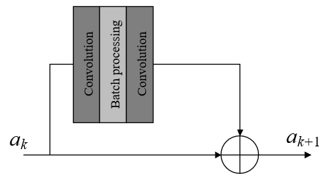
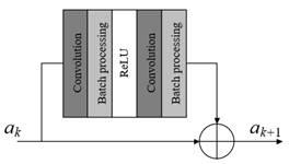
The two diagrams in Figure 5 respectively show the structure of residual unit adopted in this paper and the structure of conventional residual unit, to improve training speed, the residual unit adopted in this paper removes two regularization batch processing layers from its structure.
1) The proposed structure
2) The conventional structure
Figure 5. Structure of residual unit
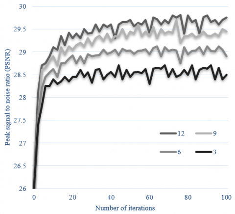
In the proposed model, several residual feature cascade modules have been set, to verify the influence of the module number on the reconstruction performance of the model, experiments were carried out during which the module number was changed to compare the model performance on sample set, Figure 6 summaries the influence of the number of residual feature cascade modules on the model’s reconstruction performance.
As can be seen from the figure, with the increase of the number of residual feature cascade modules, the reconstruction performance of the proposed model rises accordingly. The module number was set as 3, 6, 9, and 12 respectively during the comparative experiment, and the results proved that the reconstruction performance of the proposed model gets better as the module number grows. However, although increasing module number can improve model performance, it can make the model structure more complex, thereby reducing image reconstruction efficiency. After weighing the image reconstruction efficiency and the computational efficiency of the model, 9 was determined as the number of residual feature cascade modules of the proposed model.
The deep layer feature mapping module consists of three parts: long skip residual connection, hierarchical attention residual unit, and residual cascade. To verify the influence of these different parts on the reconstruction performance of the proposed model, ablation experiment was designed to verify the effectiveness of the three parts, and 4 network design schemes with or without some of the three parts were comparatively experimented on the sample set.
Figure 6. Influence of the number of residual feature cascade modules on the model’s reconstruction performance
Table 1. Influence of different module parts on network performance
|
Network design scheme |
Long skip residual connection |
Hierarchical attention residual unit |
Residual cascade |
PSNR |
|
Reference 1 |
× |
× |
× |
28.42dB |
|
Reference 2 |
√ |
× |
√ |
28.85dB |
|
Reference 3 |
× |
√ |
√ |
28.86dB |
|
Ours |
√ |
√ |
√ |
30.85dB |
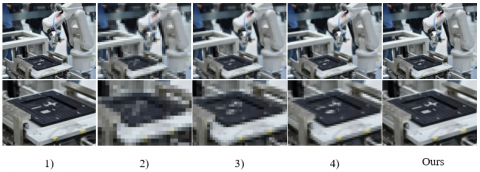
Figure 7. Image reconstruction performance of different schemes under a fixed sampling rate
According to Table 1, in cases that two of the three module parts were used or not used, the image reconstruction performance of the proposed model could still be improved, and PSNR reached 28.85 dB and 28.86 dB, respectively. In case that all three parts were used, the image reconstruction performance of the proposed model was improved further, and the PSNR reached 30.85 dB, indicating that the three module parts play a key role in enhancing the image reconstruction performance of the proposed model.
To effectively evaluate the image reconstruction performance of the proposed model, 2 indicators peak signal-to-noise ratio (PSNR) and structural similarity (SSIM) were adopted to assess the visual effect of reconstructed visual images of production equipment under different sampling rates. Three reference models were adopted in the comparative experiment, including the D-AMP model, EDSR model, and SR-CNN model. Figure 7 gives the original images and the re-constructed images of different models in case of a fixed sampling rate. As can be seen from the visual effect of sample image, overall contour features of the image had been effectively reconstructed, and there’s no obvious block in local areas of the image, which has verified that the validity of the proposed model in reconstructing image contour and restoring image details, and it outperformed other models in the experiment.
Table 2 compares the performance of different reconstruction methods under several sampling rates, and lists their PSNR and SSIM on the sample set. As can be seen from the table, under 4 sampling rates 0.05, 0.1, 0.15, and 0.2, the evaluation indicators of the proposed model showed significant improvements, which have further verified the validity of the proposed model.
Table 3 compares the image reconstruction time of different methods under different scales, and lists their reconstruction speed on sample sets of different scales. As can be seen from the table, in case of two image sizes 512×512 and 256×256, the image reconstruction time of the proposed model is shorter, which has effectively saved the consumption of hardware resource.
Table 4 compares the performance of different models under three scales of ×2,×3, and×4 in terms of PSNR and SSIM on different sample sets, according to the table, on the four sample sets coming from different sources, compared with other three models, the proposed model achieved the best image reconstruction results in terms of PSNR and SSIM under the condition of three scales, which has further verified that the proposed model outperformed the other three in terms of visual image reconstruction effect of production equipment.
Table 2. Performance of different reconstruction methods under different sampling rates
|
Model |
0.05 |
0.1 |
0.15 |
0.2 |
||||
|
PSNR |
SSIM |
PSNR |
SSIM |
PSNR |
SSIM |
PSNR |
SSIM |
|
|
D-AMP |
20.97 |
0.5712 |
23.98 |
0.6972 |
26.81 |
0.7891 |
28.32 |
0.8123 |
|
EDSR |
24.16 |
0.6992 |
25.63 |
0.7534 |
26.79 |
0.7907 |
27.52 |
0.8121 |
|
SR-CNN |
24.65 |
0.7223 |
26.59 |
0.7879 |
27.92 |
0.8223 |
28.75 |
0.8424 |
|
Ours |
29.67 |
0.8709 |
30.43 |
0.8912 |
29.36 |
0.8835 |
30.53 |
0.8905 |
Table 3. Image reconstruction time of different reconstruction methods under different scales
|
Model |
Image size |
|
|
515×515 |
256×256 |
|
|
D-AMP |
21.34 |
16.57 |
|
ReconNet |
1.72 |
0.43 |
|
NL-MRN |
92.36 |
22.21 |
|
Ours |
1.55 |
0.37 |
Table 4. Performance of different models under different scales
|
Model |
Scale factor |
Sample set 1 PSNR/SSIM |
Sample set 2 PSNR/SSIM |
Sample set 3 PSNR/SSIM |
Sample set 4 PSNR/SSIM |
|
D-AMP |
×2 |
23.67/0.9295 |
20.25/0.8687 |
29.55/0.8432 |
26.89/0.8405 |
|
×3 |
20.38/0.8681 |
27.53/0.7753 |
27.23/0.7386 |
24.47/0.7351 |
|
|
×4 |
28.45/0.8107 |
26.01/0.7029 |
25.91/0.6672 |
23.15/0.6578 |
|
|
ReconNet |
×2 |
26.67/0.9543 |
22.44/0.9068 |
21.37/0.8875 |
29.53/0.8953 |
|
×3 |
22.74/0.9091 |
29.32/0.8216 |
28.42/0.7866 |
26.25/0.7985 |
|
|
×4 |
20.42/0.8627 |
27.53/0.7514 |
26.93/0.7103 |
24.56/0.7223 |
|
|
NL-MRN |
×2 |
27.01/0.9541 |
22.76/0.9099 |
21.52/0.8940 |
29.88/0.9066 |
|
×3 |
23.03/0.9127 |
29.45/0.8273 |
28.52/0.7938 |
26.42/0.8162 |
|
|
×4 |
20.68/0.8645 |
27.73/0.7563 |
29.97/0.7123 |
24.62/0.7361 |
|
|
Ours |
×2 |
37.55/0.9523 |
33.06/0.9135 |
31.91/0.8961 |
30.78/0.9145 |
|
×3 |
33.68/0.9211 |
29.77/0.8324 |
30.84/0.8992 |
30.15/0.8793 |
|
|
×4 |
31.36/0.8824 |
31.09/0.8681 |
31.30/0.8263 |
30.62/0.8981 |
This paper studied a new visual image reconstruction method of production equipment for industrial intelligent terminals, proposed an image denoising algorithm based on hybrid statistical model, and realized noise suppression of visual image of production equipment for industrial intelligent terminals. At first, this paper made full use of the information of image features and constructed a super resolution image reconstruction model based on the fusion of hierarchical attention residual features and applied it to the visual image reconstruction of production equipment. Then, in the experiment, to figure out the influence of the number of residual feature cascade modules on the model’s reconstruction performance, 9 residual feature cascade modules were set for the proposed model, and an ablation experiment was designed to verify the effectiveness of three model parts (long skip residual connection, hierarchical attention residual unit, and residual cascade), and the results proved that the three parts play a key role in enhancing the image reconstruction performance of the model. Then, two indicators PSNR and SSIM were adopted to evaluate the visual effect of visual images of production equipment under different sampling rates, and it’s verified that the proposed model is effective in reconstructing image contour and restoring image details, and its performance outperformed other models in the experiment. At last, the model performance under different sampling rates, as well as the image reconstruction time of different models under different scales were compared, and the results of PSNR and SSIM in case of three scales ×2, ×3, ×4 on different sample sets were given, which have further verified the advantage of the proposed model over other reference models.
This study was supported by the Project of Science and Technology of Shenzhen (Grant No.: GJHZ20200731095412038 and JSGG20201102154002006).
[1] Gupta, A., Randhawa, P. (2022). Implementing industry 4.0 and sustainable manufacturing: leading to smart factory. In Industry 4.0 and Advanced Manufacturing: Proceedings of I-4AM 2022, pp. 471-482. Singapore. https://doi.org/10.1007/978-981-19-0561-2_41
[2] Casalicchio, E., Gualandi, G. (2021). ASiMOV: A self-protecting control application for the smart factory. Future Generation Computer Systems, 115: 213-235. https://doi.org/10.1016/j.future.2020.09.003
[3] Tsuzuki, R. (2021). Digital smart factory initiatives and productivity improvement in the aircraft industry. Yosetsu Gakkai Shi/Journal of the Japan Welding Society, 90(1): 44-59.
[4] Jung, G., Ha, H., Lee, S. (2021). Anomaly detection of facilities and non-disruptive operation of smart factory using kubernetes. Journal of Information Processing Systems, 17(6): 1071-1082. https://doi.org/10.3745/JIPS.01.0083
[5] Chiu, P.C., Su, K.W., Ou, T.Y., Yu, C.L., Cheng, C.Y., Hsiao, W.C., Lin, G.Y. (2021). An adaptive location-based tracking algorithm using wireless sensor network for smart factory environment. Mathematical Problems in Engineering, 2021: Article ID 4325708. https://doi.org/10.1155/2021/4325708
[6] Azarias, F.L.F., Mota, L.T.M. (2022). Logistics 4.0 for today and tomorrow: how to identify smart factory challenges and trends. In Proceedings of the 7th Brazilian Technology Symposium (BTSym’21) Emerging Trends in Human Smart and Sustainable Future of Cities, pp. 115-122. Campinas, Brazil. https://doi.org/10.1007/978-3-031-04435-9_11
[7] Peng, Q., Ren, H., Pan, C., Liu, N., Elkashlan, M. (2022). Resource allocation for uplink cell-free massive MIMO enabled URLLC in a smart factory. IEEE Transactions on Communications., 71(1): 553-568. https://doi.org/10.1109/TCOMM.2022.3224502
[8] Baranwal, G., Vidyarthi, D.P. (2021). Computation offloading model for smart factory. Journal of Ambient Intelligence and Humanized Computing, 12: 8305-8318. https://doi.org/10.1007/s12652-020-02564-0
[9] Sun, X., Yang, Y., Liu, C., Guo, H. (2015). Design and development of near field communication intelligent data acquisition terminal system in fresh agricultural product supply chain. Transactions of the Chinese Society of Agricultural Engineering, 31(8): 200-206. https://doi.org/10.3969/j.issn.1002-6819.2015.08.029
[10] Liu, Y., Chen, Y., Tzeng, G.H. (2017). Identification of key factors in consumers’ adoption behavior of intelligent medical terminals based on a hybrid modified MADM model for product improvement. International Journal of Medical Informatics, 105: 68-82. https://doi.org/10.1016/j.ijmedinf.2017.05.017
[11] Gao, L., Xiao, Q., Liu, C.X., Ding, J.L., Chai, T.Y. (2016). Beneficiation production index optimization decision system based on intelligent mobile terminal and cloud computing. Jisuanji Jicheng Zhizao Xitong/Computer Integrated Manufacturing Systems, CIMS, 22(7): 1821-1829. https://doi.org/10.13196/j.cims.2016.07.021
[12] Yang, B., Pang, Z., Wang, S., Mo, F., Gao, Y. (2022). A coupling optimization method of production scheduling and computation offloading for intelligent workshops with cloud-edge-terminal architecture. Journal of Manufacturing Systems, 65: 421-438. https://doi.org/10.1016/j.jmsy.2022.10.002
[13] Wang, W., Wang, Y. (2022). Research on image capture technology of intelligent terminal and multi exposure fusion to improve the resilience of agriculture production systems. Journal of Commercial Biotechnology, 27(2): 46-56. https://doi.org/10.5912/jcb1045
[14] Schmitt, R.H., Wolfschläger, D., Masliankova, E., Montavon, B. (2022). Metrologically interpretable feature extraction for industrial machine vision using generative deep learning. CIRP Annals, 71(1): 433-436. https://doi.org/10.1016/j.cirp.2022.03.016
[15] Sungho, K., Wangheon, L. (2022). Guest editorial: machine vision and ai+x-based industrial applications. Journal of Institute of Control, Robotics and Systems, 28(10): 847.
[16] Wang, H., Lu, R., Yu, D. (2022). Machine vision nondestructive inspection system Assisted by industrial IoT supervision mechanism. Mathematical Problems in Engineering, 2022: Article ID 8449518. https://doi.org/10.1155/2022/8449518
[17] Mirbod, M., Ghatari, A.R., Saati, S., Shoar, M. (2022). Industrial parts change recognition model using machine vision, image processing in the framework of industrial information integration. Journal of Industrial Information Integration, 26: 100277. https://doi.org/10.1016/j.jii.2021.100277
[18] Lauzon-Gauthier, J., Duchesne, C., Tessier, J. (2022). Machine vision sensor based on image texture analysis applied to industrial anode paste. In Light Metals, 2022: 834-842. https://doi.org/10.1007/978-3-030-92529-1_110
[19] Lyu, C., Zhang, M., Li, B., Liu, Y., Lin, X. (2022). High reliability pipeline leakage detection based on machine vision in complex industrial environment. IEEE Sensors Journal, 22(21): 20748-20760. https://doi.org/10.1109/JSEN.2022.3206456
[20] Xiang, S. (2021). Industrial automatic assembly technology based on machine vision recognition. Manufacturing Technology Engineering Science and Research Journal, 21: 141-148. https://doi.org/10.21062/mft.2021.018
[21] Ye, T., Zhao, L. (2021). Design of industrial robot teaching system based on machine vision. In 2021 IEEE 5th Information Technology, Networking, Electronic and Automation Control Conference (ITNEC), 5: pp. 279-284. Xi'an, China. 10.1109/ITNEC52019.2021.9586814
[22] Yang, C. (2021). Research on grasping method of industrial robot based on deep learning and machine vision. In Journal of Physics: Conference Series, 1992(3): 032039. https://doi.org/10.1088/1742-6596/1992/3/032039
[23] Li, M., Jia, J., Lu, X., Zhang, Y. (2021). A method of surface defect detection of irregular industrial products based on machine vision. Wireless Communications and Mobile Computing, 2021: Article ID 6630802. https://doi.org/10.1155/2021/6630802
[24] Jin, Z., Liu, L., Gong, D., Li, L. (2021). Target recognition of industrial robots using machine vision in 5G environment. Frontiers in Neurorobotics, 15: 624466. https://doi.org/10.3389/fnbot.2021.624466
[25] Tang, H., Hu, G., He, W., Tu, Q. (2022). Improved anomaly detection based on image reconstruction and global template features for industrial products. In Journal of Physics: Conference Series, 2166(1): 012062. https://doi.org/10.1088/1742-6596/2166/1/012062
[26] Fu, L., Jiang, H., Wu, H., Yan, S., Wang, J., Wang, D. (2023). Image super-resolution reconstruction based on instance spatial feature modulation and feedback mechanism. Applied Intelligence, 53(1): 601-615. https://doi.org/10.1007/s10489-022-03625-x
[27] Liu, Y., Zhang, J., Zhang, Y. (2023). Hyperspectral reconstruction from a single textile RGB image based on the generative adversarial network. Textile Research Journal, 93(1-2): 307-316. https://doi.org/10.1177/00405175221118105
[28] Zhang, N. (2023). Colour image reconstruction in indoor space based on machine vision. International Journal of Information and Communication Technology, 22(2): 117-132. https://doi.org/10.1504/IJICT.2023.128743