Chettukrindi Mohammad Aslam* | Donti Satya Narayana | Kesari Padma Priya
© 2022 IIETA. This article is published by IIETA and is licensed under the CC BY 4.0 license (http://creativecommons.org/licenses/by/4.0/).
OPEN ACCESS
A new segmentation method for medical image with intensity clustering is enclosed. In the intended approach, an improved K-means and EM algorithm are combined to develop a hybrid strategy for better clumping. The intended advent aims to exploit the ability of providing well distributed clump of K-means and the closeness of clumps provided by EM. The introductory clumps are provided by the improved K-means algorithm. This introductory clumping process outcomes in canters which are distributed in the given data. These canters form the introductory variable for EM, which afterwards uses them and repeats to find the local maxima. Experiments for synthetic and real images make evident the feasibility and superiority of the projected model.
K-means algorithm, EM algorithm, Gaussian mixture model
Image segmentation is one of the most deliberate problems in image analytics. The least complex procedures depend on a histogram of the image, that doesn’t have any spatial information. Hence, the classification remains constant to transposition of the pixels, neglecting the spatial dependence in image segmentation [1]. They require to include spatial data lead to the disclosure of techniques using neighbourhood [2, 3]. MRF theory is wont to shape the inherent spatial dependences [4, 5]. These models have been utilized in diverse maximum a posteriori (MAP) method for image restoration and segmentation [6].
When the MRF theory was the area of image analytics during 1980s. Geman and Geman [4] and Besag [7] applied MRFs to image segmentation. Analogues to the effort done by Geman and Geman [4], Geiger and Girosi [8] also combined a second MRF to the aboriginal MRF for plane restoration. Similarly, Jeng and Woods [9] and Molina et al. [10] introduce edge MRF with intensity mechanism.
Today, clustering algorithms are notable analytic devices for image segmentation. Being, the K-means is the best exploited method of the previous work which is fast, strong and less demanding to comprehend. but, the principal disadvantage of the K-means is initially the number of clumps should be well-known and should be provided as an input as. This paper deliberates the issue of the appraisal of the number of clumps for image segmentation and intends a new advent that depends on a hybrid technology of K-means and EM algorithm. The formulated model is experimented on Breast, Brain MRI Images and continent images of size. The results are better than conventional methods like k-means, Fuzzy C-Means, Watershed segmentation methods.
In this paper, the interaction of different image segmentation techniques is first analyzed. Next, the clustering characteristics of image pixels and paper are researched. And the reasons of the drawbacks of not to detect portions of image and different kinds of papers are studied. After that, the new algorithm for image detection is introduced. Then, the effective data processing methods are presented. As a result, high-quality image detection on porous paper is achieved, and then the image ridges characteristics are obtained, which provides quantitative evidences for image analytics.
An image is a collection of multi-dimensional information and distributing it into various segments in accordance with some similarity norm is named Clustering. K-Means is a significant clustering algorithm that is extensively opted to distinct fields of functions inclusive of computer vision, astronomy and image segmentation. But straight K-means algorithm needs time comparative to the multiplication of number of patterns and clusters per iteration.
The K-means [11] is the basic clustering algorithm endorsed for the image segmentation due to the clustering efficacy and simplicity of application. Adaptive genetic algorithm for real time images employs k-means clustering to generate a set of individuals randomly by genetic process, Machine learning is a text classification algorithm which also uses k-means for feature selection [12]. A Traffic flow model where day-by-day traffic flow diagrams are generated by k-means and Frichet distance based clustering is used to link the diagrams [13]. To surmount the issues induced by the nosy method for attaining the plasma time-activity curve (PTAC) required for positron emission tomography (PET), Zheng et al. [14] presents a hybrid clustering method (HCM) using k-means clustering and polynomial regression mixture model. Ranjbaran et al. [15] defines a new algorithm to differentiate the VOR data into different intervals accordingly. Clustering method can have much improved outcomes of segmentation. But over-segmentation is the headache which should be resolved and feature extraction is a significant aspect of clustering.
The FCM algorithm [16], the best clustering algorithm for segmentation of image. FCM can be developed as the minimization function as follows:
$J_{f c m}=\sum_{i=1}^N \sum_{j=1}^C u_{i j}^m\left\|x_i-c_j\right\|^2$ (1)
where, u=membership function, C=centre of the cluster.
For medical image analytics, Mohamed et al. [17] introduced a new FCM algorithm. They used the spatial data for the similarity measure. Its subtlety towards the non-prescriptive introductory centres and its high computing complexity are the deficiencies of the FCM algorithm [18]. Therefore, Ahmed et al. [19] proposed a different closeness measure in the Bias-Corrected FCM (BCFCM) algorithm. It achieves a good accomplishment by defining an objective function. Later number of researchers alters the objective functions and built up various potent FCM algorithms for image segmentation [20-24]. These algorithms shown a better accomplishment compared to the standard FCM algorithm. Yet, some of the techniques [20, 22, 23] rely upon a fixed spatial factor that has to be modified in accordance with the real-time utilization. The new likeliness measure uses the local and spatial intensity data. hence gives superior performance, reduces the blurring effect. Even though, the blurring problems still exist, and there is a need for experimentally adjusted parameters.
This paper introduces a novel MRF clumping approach to represent the noise problem.
2.1 Proposed method
The present advent is an improved K -means process and Expectation and Maximization method (EM) are combined to present a combined strategy for better clumping. The present method concentrates on exploiting the ability of providing well distributed clump of K-means and the closeness of clumps provided by EM. The introductory clumps are given by the improved K-means method. This underlying grouping process outcomes in centres that are generally around the data. Thus formed centres create the introductory variable for EM and finds maximum likelihood (ML) of them. Vulnerable to K-means, in EM the numbers of groups which required are foregone. It is instated with values for obscure (concealed) factors. Since EM utilizes maximum likelihood, it probably converges to local maxima, in the neighbourhood of initial values. So, selection of introductory values is crucial for EM. Anyhow, the EM method functions great on clumping information, by knowing the number of clumps.
Given a set {xi}, where xi is the gray value of the ith pixel represented as i.i.d and N is the total number of pixels. GMM represents a mixture model containing Gaussian density (c) components with the parameters in the kth component. In GMM, the probability density of xi developed as:
$p\left(x_i \mid \pi, \theta\right)=\sum_{k=1}^c \pi_k p\left(x_i \mid \theta_k\right) p\left(x_i \mid \theta_k\right)$ (2)
where, i={1, 2, 3, …} is the parameters of all the components and πk is the mixing weight of the kth component, satisfying and. The kth Gaussian is represented by:
$p\left(x_i \mid \theta_k\right)=\frac{1}{\sqrt{(2 x)\left|\sum_k\right|}} \exp \left(-\frac{\left(x_i-u_k\right)^T \sum_k^{-1}\left(x_i-u_k\right)}{2}\right)$ (3)
where, µk and Σk are the mean and the covariance matrix, respectively. The parameters {θ, π} can repetitively predicted by exaggerating the similarity function using the proposed hybrid Expectation-Maximization.
The k-means algorithm generates k-points as introductory centroids randomly, k is a user defined parameter. Now each point is allotted to the closest centroid group. Then the centroid of each clique is amended by considering the average of the points of each clump. The distance between distributed points and centroids can be found by Euclidean.
In the intended formulation, a computationally simple advent is advised to identify better introductory clumps and hence increasing conduct of the clumping phenomena.
Expectation maximization clumping calculates the probability densities of the classes using the Expectation Maximization (EM) process. It is based on identifying the highest probability parameter assessment, when the data model looks upon certain hidden factors. In this intended advent, the introductory clumps are find using improved K –means method and alternate steps of Expectation (E) and Maximization (M) are executed repeatedly until the converged outcome is achieved. The E-step figure-outs an expectation of the homogeneity by combining the concealed factors whenever they detected, and maximization (M) step, calculates the highest similarity assessment of the parameters by increasing the homogeneity found on the last E-step. The previous M-step parameters are used to commence next E-step, and the procedure is rehashed till the accomplishment of the convergence.
Consider a set of data {x(1), x(2),……x(m)} and model p(x, z), where z is the hidden factor.
$l(\theta)=\sum_1^m \log \sum_z p(x ; z ; \theta)$ (4)
$\left.=\sum_1^m \log \sum_{\mathrm{z}} p(x ; z ; \theta), \theta\right)$ (5)
From Eq. (5), the log likelihood is represented in x, z and θ. where as z, the unknown hidden factor, then we use estimations rather. These estimations were in the form of E & M steps specified above and developed as follows:
E Step, for each $i$ :$Q_i\left(z^{(i)}\right)=P\left(z^{(i)} / x^{(i)} ; \theta\right)$ (6)
M Step, for all $z$ :$\theta:=\arg \max _\theta \sum_i \sum_{z^{(i)}} Q_i\left(z^{(i)}\right)$ (7)
where, Qi=posterior distribution of z(i)’s given the x(i).
To include the spatial data into GMM, a new GMM is formulated using the MRF model as a precedent. Deviating the GMM, every pixel i in Modified GMM is defined with its probability vector πi=(πi1, πi2,…, πic)T where π represents the likeliness of the ith pixel appertaining to the kth clump. In new GMM, the mixture model of x is defined as:
$p\left(x_i \mid \pi, \theta\right)=\sum_{k=1}^c \pi_i^k p\left(x_i \mid \theta_k\right) p\left(x_i \mid \theta_k\right)$ (8)
where, p(xi|θk)=Gaussian distribution with parameters θk={μk,Σk}. In order to consider the spatial dependence, the prior distribution of π is represented by the MRF model by the Gibbs density function:
$\hat{H}_{\text {MMSE }}(k)=R_{H(k) Y(k)} R_{Y(k) Y(k)}^{-1} Y(k)$ (9)
where, Z=normalizing constant and β=regularization parameter. VNi(π) is the clique potential function of the pixel label vectors πm within the vicinity Ni of the ith pixel,
$V_{N_i}(\pi)=\sum_{m \in N_i}\left|\pi_i-\pi_m\right|^2\left|\pi_i-\pi_m\right|^2$ (10)
Notice that the π={π1, π2, …, πk} in GMM is distributed by all pixels, rather in Modified GMM πi is distinct for each pixel i and based on its neighbouring pixels. In Modified GMM, the modified EM process is used to get the maximum a posteriori (MAP) estimation of the parameters.
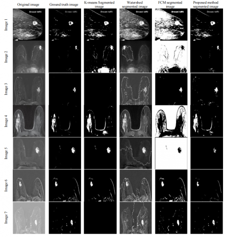
Figure 1. Simulation results of various medical images
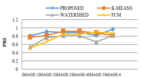
Table 1. Probability Rand Index (PRI) simulation
|
|
PROPOSED |
K-MEANS |
WATERSHED |
FCM |
|
IMAGE-1 |
0.81 |
0.7744 |
0.5387 |
0.5104 |
|
IMAGE-2 |
0.91 |
0.8196 |
0.764 |
0.667 |
|
IMAGE-3 |
0.89 |
0.92 |
0.81 |
0.85 |
|
IMAGE-4 |
0.89 |
0.92 |
0.81 |
0.85 |
|
IMAGE-5 |
0.82 |
0.88 |
0.66 |
0.9 |
|
IMAGE-6 |
0.97 |
0.82 |
0.82 |
0.87 |
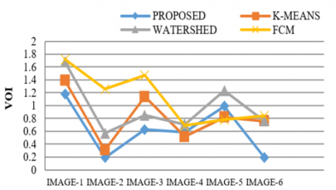
Table 2. Variation of Information (VOI)
|
|
PROPOSED |
K-MEANS |
WATERSHED |
FCM |
|
IMAGE-1 |
1.18 |
1.39 |
1.68 |
1.72 |
|
IMAGE-2 |
0.19 |
0.31 |
0.57 |
1.26 |
|
IMAGE-3 |
0.63 |
1.14 |
0.85 |
1.47 |
|
IMAGE-4 |
0.59 |
0.52 |
0.71 |
0.69 |
|
IMAGE-5 |
0.99 |
0.82 |
1.23 |
0.78 |
|
IMAGE-6 |
0.19 |
0.76 |
0.76 |
0.84 |
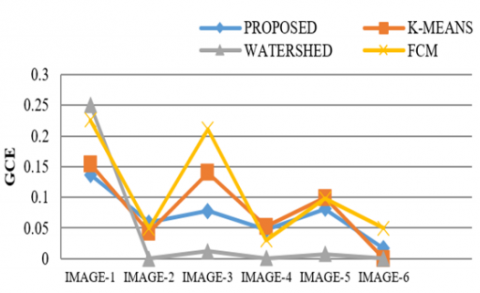
Table 3. Global Consistency Error (GCE)
|
|
PROPOSED |
K-MEANS |
WATERSHED |
FCM |
|
IMAGE-1 |
0.1366 |
0.154 |
0.2509 |
0.2259 |
|
IMAGE-2 |
0.0591 |
0.0427 |
0.00018 |
0.0498 |
|
IMAGE-3 |
0.078 |
0.14 |
0.0123 |
0.211 |
|
IMAGE-4 |
0.047 |
0.052 |
0.0005 |
0.03 |
|
IMAGE-5 |
0.081 |
0.099 |
0.0073 |
0.098 |
|
IMAGE-6 |
0.017 |
0 |
0 |
0.05 |
Table 4. Jaccord Index (JID)
|
|
PROPOSED |
K-MEANS |
WATERSHED |
FCM |
|
IMAGE-1 |
0.5171 |
0.4367 |
0.1467 |
0.0626 |
|
IMAGE-2 |
0.6494 |
0.055 |
0.0978 |
0 |
|
IMAGE-3 |
0.66 |
0.6193 |
0.35 |
0.7833 |
|
IMAGE-4 |
0.59 |
0.456 |
0.489 |
0 |
|
IMAGE-5 |
0.66 |
0.96 |
0.7 |
0 |
|
IMAGE-6 |
0.68 |
0.92 |
0.41 |
0.68 |
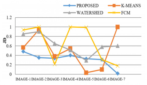
Table 5. Jaccord Distance (JD)
|
|
PROPOSED |
K-MEANS |
WATERSHED |
FCM |
|
IMAGE-1 |
0.4828 |
0.5632 |
0.8532 |
0.9373 |
|
IMAGE-2 |
0.3505 |
0.9449 |
0.9021 |
1 |
|
IMAGE-3 |
0.3392 |
0.38 |
0.65 |
0.2166 |
|
IMAGE-4 |
0.4 |
0.5439 |
0.51 |
1 |
|
IMAGE-5 |
0.33 |
0.033 |
0.29 |
0.99 |
|
IMAGE-6 |
0.31 |
0.1 |
0.58 |
0.31 |
Table 6. Peak Signal to Noise Ratio (PSNR)
|
|
PROPOSED |
K-MEANS |
WATERSHED |
FCM |
|
IMAGE-1 |
35.93 |
32.7 |
17.61 |
8.164 |
|
IMAGE-2 |
59.96 |
25.3 |
31.51 |
1.4378 |
|
IMAGE-3 |
43.4 |
46.39 |
30.57 |
49.59 |
|
IMAGE-4 |
37.72 |
31.94 |
33.29 |
4.094 |
|
IMAGE-5 |
44.32 |
66.95 |
42.06 |
0.089 |
|
IMAGE-6 |
44.57 |
57.77 |
29.73 |
41.01 |
We perform experiment on different images from the medical dataset. A set of the images are considered in this paper. Then we tried to find out which segmentation algorithm is best by considering various performance evaluation parameters. For this we take image and image mask from Berkeley Database. Ground truth is obtained by superimposing the image mask on original image. Proposed technique is compared with Watershed, K-Means, and FCM Segmentation methods with results shown in Graph 1.
The Proposed technique has been experimented over a range of 8-bit Gray scale images, which gives one layer image from 0-255 scales. To validate the efficiency of the segmentation technique using the projected technique, a set of images of various types were tested. Exploratory outputs represent the framework is fit for helping the radiologists in the understanding of scanned images. The simulation results of various medical images for the discussed algorithms have been represented in Figure 1. The execution assessment of four techniques has been pictured in the table with corresponding graphs. Tables 1 to 6 shows the PRI, GCE, VOI, JID, JD & PSNR of the Proposed, Watershed, k-Means and FCM based Segmentation techniques of different Images. It shows PRI, JID and PSNR of the projected method has higher values than the others and VOI, GCE and JD of proposed method is lower than the other methods. So, using PRI, GCE, VOI, JID, JD, and PSNR we wrap-up that proposed modified model is better than others. The small values of Variation of information and global consistency error indicate that difference between original image verses the processed image is Minimum. Similarly, the higher values of RAND INDEX, JACCORD INDEX and SIGNAL to NOISE RATIO are high indicating that the signal strength of region of interest is high. This represents the exact location and size of the bosom in the output image is same as ground truth image. The proposed method produces the better outcome than FCM, Watershed and K-Means techniques. Further comparing the plotted values in Graph 2 to Graph 6 of the same image in Table 1, it is apparent that the values clearly reflect the levels of seriousness of the disease. For instance, the plotted values for PRI, JID, JD demonstrate that the seriousness of disease in these individual images is too high, while the values for VOI, JID demonstrate that the seriousness of malignancy in these respective images is moderate and the values for PRI show that the seriousness of growth in these respective images is low.
In the three prior mentioned methods, the level of severity of cancer is not clearly reflected in PRI and is due to the values for k-means, FCM and watershed (Table 1) are either too low or too high. In the projected method, the deficiency can be extracted more accurately and is used on various mammograms applications.
Graph 1. PRI
Graph 2. Variation of Information (VOI)
Graph 3. GCE
Graph 4. JID
Graph 5. JD
Graph 6. PSNR
Evaluation measures are an efficient way to analyse the performance of existing and proposed algorithms. The performance evaluation of the intended model in comparison with current methods is analysed based on parameters and their graphical representations. Various parameters like Probability Rand Index, Variation of Information, Global Consistency Error, Jaccord Index, Jaccord Distance, and Peak Signal to Noise Ratio have been considered and their corresponding plots have been drawn. Table 1, 4 and 6 shows the PRI, JID & PSNR of the proposed technique is higher than the K-Means, Watershed & FCM Based segmentation methods. Table 2, 3, and 5 shows the VOI, GCE & JD of Proposed technique is low as compare to other methods. Thus, the proposed algorithm is proved to be better compared to the existing algorithms [25, 26].
The early detection of breast cancer in women is mammography. The illustration of mammograms greatly depends on radiologist’s assessment. The formulated model is experimented on Breast, Brain MRI Images and continent images of size. The results are better than conventional methods like k-means, Fuzzy C-Means, Watershed segmentation methods. The assets of the formulated hybrid method over other methods are that there is no guarantee for optimal clustering by k-means and by combining the advantage of maximum likelihood of the EM, we will get satisfactory results using the hybrid model for images with histogram of unimodal or multimodal distribution. But for the noise sensitive images, there may be chances of enhancing the image details.
[1] Wilson, R., Spann, M. (1988). Image Segmentation and Uncertainty. Research Studies Press Ltd.
[2] Hummel, R.A., Zucker, S.W. (1983). On the foundations of relaxation labeling processes. IEEE Transactions on Pattern Analysis and Machine Intelligence, 5(3): 267-287. https://doi.org/10.1109/TPAMI.1983.4767390
[3] Kittler, J., Föglein, J. (1983). A general contextual classification method for segmentation. In Proc. 3th Scandinavian Conf. Im. Analysis, pp. 90-95.
[4] Geman, S., Geman, D. (1984). Stochastic relaxation, Gibbs distributions, and the Bayesian restoration of images. EEE Transactions on Pattern Analysis and Machine Intelligence, 6(6): 721-741. https://doi.org/10.1109/TPAMI.1984.4767596
[5] Besag, J. (1990). Towards Bayesian Image Analysis. J.G. McWhirter (Ed.), Mathematics in Signal Processing, vol. II, Clarendon Press, Oxford.
[6] Chellappa, R., Jain, A. (1993). Markov Random Fields: Theory and Applications. Academic Press, New York.
[7] Besag, J. (1986). On the statistical analysis of dirty pictures. Journal of the Royal Statistical Society: Series B (Methodological), 48(3): 259-279. https://doi.org/10.1111/j.2517-6161.1986.tb01412.x
[8] Geiger, D., Girosi, F. (1991). Parallel and deterministic algorithms from MRFs: Surface reconstruction. IEEE Transactions on Pattern Analysis & Machine Intelligence, 13(5): 401-412. https://doi.org/10.1109/34.134040
[9] Jeng, F.C., Woods, J.W. (1991). Compound Gauss-Markov random fields for image estimation. IEEE Transactions on Signal Processing, 39(3): 683-697. https://doi.org/10.1109/78.80887
[10] Molina, R., Mateos, J., Katsaggelos, A.K., Vega, M. (2003). Bayesian multichannel image restoration using compound Gauss-Markov random fields. IEEE Transactions on Image Processing, 12(12): 1642-1654. https://doi.org/10.1109/TIP.2003.818015
[11] Rajkumar, P., Balamurgan, V., Mishra, P. (2016). Adaptive genetic algorithm for a real time medical images. In 2016 Online International Conference on Green Engineering and Technologies (IC-GET), Coimbatore, India, pp. 1-5. https://doi.org/10.1109/GET.2016.7916803
[12] Neethu, K.S., Jyothis, T.S., Dev, J. (2016). Text classification using KM-ELM classifier. In 2016 International Conference on Circuit, Power and Computing Technologies (ICCPCT), Nagercoil, India, pp. 1-5. https://doi.org/10.1109/ICCPCT.2016.7530338
[13] Gu, Z., Saberi, M., Sarvi, M., Liu, Z. (2016). Calibration of traffic flow fundamental diagrams for network simulation applications: A two-stage clustering approach. In 2016 IEEE 19th International Conference on Intelligent Transportation Systems (ITSC), Rio de Janeiro, pp. 1348-1353. https://doi.org/10.1109/ITSC.2016.7795732
[14] Zheng, X., Tian, G., Huang, S.C., Feng, D. (2010). A hybrid clustering method for ROI delineation in small-animal dynamic PET images: Application to the automatic estimation of FDG input functions. IEEE Transactions on Information Technology in Biomedicine, 15(2): 195-205. https://doi.org/10.1109/TITB.2010.2087343
[15] Ranjbaran, M., Smith, H.L., Galiana, H.L. (2015). Automatic classification of the vestibulo-ocular reflex nystagmus: integration of data clustering and system identification. IEEE Transactions on Biomedical Engineering, 63(4): 850-858. https://doi.org/10.1109/TBME.2015.2477038
[16] Bezdek, J.C. (2013). Pattern Recognition with Fuzzy Objective Function Algorithms. Springer Science & Business Media.
[17] Mohamed, N.A., Ahmed, M.N., Farag, A. (1998). Modified fuzzy c-mean in medical image segmentation. In Proceedings of the 20th Annual International Conference of the IEEE Engineering in Medicine and Biology Society. Vol.20 Biomedical Engineering Towards the Year 2000 and Beyond (Cat. No.98CH36286), Hong Kong, China, pp. 1377-1380. https://doi.org/10.1109/IEMBS.1998.747137
[18] Davé, R.N., Krishnapuram, R. (1997). Robust clustering methods: A unified view. IEEE Transactions on Fuzzy Systems, 5(2): 270-293. https://doi.org/10.1109/91.580801
[19] Ahmed, M.N., Yamany, S.M., Farag, A.A., Moriarty, T. (1999). Bias field estimation and adaptive segmentation of MRI data using a modified fuzzy C-means algorithm. In Proceedings. 1999 IEEE Computer Society Conference on Computer Vision and Pattern Recognition (Cat. No PR00149), Fort Collins, CO, USA, pp. 250-255. https://doi.org/10.1109/CVPR.1999.786947
[20] Tolias, Y.A., Panas, S.M. (1998). Image segmentation by a fuzzy clustering algorithm using adaptive spatially constrained membership functions. IEEE Transactions on Systems, Man, and Cybernetics-Part A: Systems and Humans, 28(3): 359-369. https://doi.org/10.1109/3468.668967
[21] Liew, A.W.C., Leung, S.H., Lau, W.H. (2000). Fuzzy image clustering incorporating spatial continuity. IEE Proceedings-Vision, Image and Signal Processing, 147(2): 185-192. https://doi.org/10.1049/ip-vis:20000218
[22] Pham, D.L. (2001). Spatial models for fuzzy clustering. Computer Vision and Image Understanding, 84(2): 285-297. https://doi.org/10.1006/cviu.2001.0951
[23] Szilagyi, L., Benyo, Z., Szilágyi, S.M., Adam, H.S. (2003). MR brain image segmentation using an enhanced fuzzy C-means algorithm. In Proceedings of the 25th Annual International Conference of the IEEE Engineering in Medicine and Biology Society (IEEE Cat. No. 03CH37439), Cancun, Mexico, pp. 724-726. https://doi.org/10.1109/IEMBS.2003.1279866
[24] Cai, W., Chen, S., Zhang, D. (2007). Fast and robust fuzzy C-means clustering algorithms incorporating local information for image segmentation. Pattern Recognition, 40(3): 825-838. https://doi.org/10.1016/j.patcog.2006.07.011
[25] Ariyapadath, S. (2021). Plant leaf classification and comparative analysis of combined feature set using machine learning techniques. Traitement du Signal, 38(6): 1587-1598. https://doi.org/10.18280/ts.380603
[26] Ozdemir, C., Gedik, M.A., Kaya, Y. (2021). Age estimation from left-hand radiographs with deep learning methods. Traitement du Signal, 38(6): 1565-1574. https://doi.org/10.18280/ts.380601