Amin Jarrah* | Sereen Amri
© 2022 IIETA. This article is published by IIETA and is licensed under the CC BY 4.0 license (http://creativecommons.org/licenses/by/4.0/).
OPEN ACCESS
There is a need for fast, accurate, and real-time algorithms to detect brain tumors effectively to support the physician’s decision-making for treatment purposes. A brain tumor is a life-threatening uncontrolled growth of cells and tissues that may cause death due to inaccurate and late detection. K-means clustering is one of the clustering techniques that is widely used in brain tumor detection, but it has some drawbacks such as dependency on initial centroid values and a tendency to fall on local optima. This research proposes a new model that uses grey wolf optimization to find the optimal value of K (clusters number) of the k-means algorithm to avoid local optima. A parallel implementation of the K-means clustering algorithm on a field-programmable gate array (FPGA) is also proposed to enhance the performance by reducing the processing time and the power consumption. Moreover, the proposed algorithm is implemented using the Vivado HLS tool on Xilinx Kintex7 XC7K160t FPGA 484-1 where different optimization techniques are adopted and applied, such as loop unrolling, loop pipelining, dataflow, and loop merging. The achieved speed-up of the parallel implementation compared with sequential implementation was 88.17, where the obtained average clustering accuracy was 97.11%.
brain tumor detection, grey wolf optimization, k-means clustering algorithm, optimization techniques, parallel implementation
All human body activities are controlled by the brain, including intelligence, memory, speech, senses, etc. [1]. The brain consists of three types of tissues, including grey matter, white matter, and cerebrospinal fluid [1]. A brain tumor is an abnormal and uncontrolled growth of brain cells. It is a life-threatening disease that can be primary or secondary due to metastasis from other organs in the body. It’s classified into two types: malignant and benign [1]. The Magnetic Resonance Imaging technique MRI is the preferred imaging technique to detect brain tumors [2] since it’s widely used in hospitals for diagnosis, treatment, and follow-up disease [2]. It is used to create a picture of the anatomy and physiology of body organs. MRI has the advantage of being non invasive diagnostic tool as it does not use radiation. Thus, it’s commonly used to image soft tissues such as the brain, where it detects changes in the brain, including bleeding and tumors [2].
Early detection of brain tumors helps in accelerating the treatment and saving human lives [3]. There are many brain tumor detection algorithms that are proposed to help in the diagnosis and treatment processes [3]. K-means is one of these algorithms [3]. It is an unsupervised, simple, and practicable algorithm that classifies the observations into classes. It was chosen because it is efficient and does not necessitate significant effort in data preprocessing, training, and testing [3]. However, K-means has some drawbacks, such as the dependency on initial centroid values, the large number of iterations, determining the number of clusters and a tendency to fall into local optima [4]. Therefore, the Grey Wolf Optimization (GWO) technique [5] was adopted and applied to determine the optimal number of clusters. It’s an optimization technique that is inspired by the behavior of grey wolves and their strategies for eating and hunting [5]. This will help in optimizing the accuracy by avoiding falling into local optimum and improving the processing speed.
However, the detection of brain tumors from MRI images is a computationally intensive task, especially when the image size increases. It requires processing of a massive amount of data known as Big Data, especially for processing MRI for brain tumor detection which needs high-speed processing to analyze data [3]. Therefore, a parallel implementation of the proposed K-means based on GWO was proposed and implemented on the FPGA parallel platform. This means that more than one section of a system may operate with a different set of data concurrently to improve the execution time [6]. However, the FPGA needs a long time for designing, implementation, and validation processes since it requires knowledge of digital systems and underlying architectures [6]. Xilinx FPGA has a powerful tool called the Vivado HLS tool which can be used to overcome these constraints [7]. Therefore, the Vivado High-Level Synthesis tool for synthesis and simulation was adopted and used. It’s a tool that is used for configuring the FPGA and converting the C family code into a hardware description language. So, the proposed algorithm was implemented on the Vivado HLS tool where different optimization techniques were adopted and applied.
The remainder of this paper is organized as follows: Section I provides an overview of the topic. Section II discusses the related work. Section III explains the K-means algorithm and its operation. Section IV shows a brief description of the Grey Wolf Optimization, while Section V provides an explanation of the FPGA and Vivado HLS tool, Section ⅤI presents the proposed methodology with a detailed explanation, and Section ⅥI presents and analyzes the results obtained from the described implementation. Finally, Section ⅦI concludes the results and remarks of the work.
In the last few years, many researchers have proposed many parallel implementations of the K-means algorithm. A completely parallel implementation of the K-means clustering technique was developed on FPGA [8]. To accelerate processing time and separate huge amounts of data (Big Data) into K clusters, they used the Euclidean distance metric to calculate the similarity between the data and the initial centroid of each cluster to determine to which cluster the data belongs. They reached a performance level of more than 53 million data points processed per second. In the study of Hema and Madhavi [9], accurate results of tumor segmentation on MRI images with FPGA-based K-means clustering are obtained where there is no information regarding the speed-up or the image size. Jaroš et al. [10] presented a method for speeding up K-means clustering, which is used in medical image segmentation. They used many integrated circuit MIC architectures with the Intel Xeon Phi coprocessor to perform a parallel implementation of the algorithm. They compared MIC with CPU and GPU on Computed Tomography (CT) images of the human body. A parallel implementation of 2D image clustering has been proposed on an FPGA using the moving window technique [11]. The authors used a multi-core FPGA to reduce the required processing time of the clustering technique. The implementation of the K-means clustering algorithm on FPGA has been proposed in the field of bioinformatics to analyze microarray data [12]. Microarray data is a technique used by biologists to perform many genome experiments. Using FPGA in this domain is very effective because of the huge amount of data that needs to be analyzed. They used five K-means cores on Xilinx Virtex4 XC4VLX25 FPGA and achieved a speed-up of 51.7 times. All previous works have a limitation where the value of K was not accurate since it was selected randomly and sometimes based on expectation, which may fall into local optima. Therefore, in this research, we adopted and applied the Grey Wolf Optimization (GWO) technique to determine the optimal number of clusters (K) and overcome the above mentioned limitations.
Many researchers use metaheuristic algorithms to overcome the shortcomings of classical K-means algorithms. GWO is used in the study [13] as a solution to the K-means algorithm's problems. The authors combined GWO with K-means clustering to solve a capacitated vehicle routing problem [13]. Each wolf searches for a set of centroids based on cluster number to avoid random initialization of centroids. The authors [14] proposed Grey Wolf Algorithm-based Clustering (GWAC), where the search capability of GWO is used to search for optimal initial centroids of K-means clustering.
K-means clustering is a widely used algorithm that divides datasets into groups or "clusters" based on similarity metrics [8]. Each data point is assigned to one cluster based on the similarity between this data point and the cluster centroid [8]. Supposing that we have a dataset $X$ defined in Eq. (1), it consists of $n$ data points that need to be clustered into $\mathrm{K}$ clusters [8] where each data point $P$ should be assigned to one cluster.
$X=(p 1, p 2, p 3 \cdots, p n)$ (1)
Firstly, the number of clusters K must be determined. As mentioned above, in traditional K-means, K is determined randomly. Accordingly, the GWO algorithm is adopted and used to help in finding the optimal value of K since the K value has a direct impact on the accuracy of the results of the K-means algorithm. Then, each cluster assigns an initial centroid where C is the set of centroids based on Eq. (2) [8]. In the traditional K-means, cluster centroids are initialized randomly. This makes the result of clustering dependent on the first centroids, which leads to a local optima problem [15]. However, a mathematical model is adopted and used based on Eq. (3) to initialize the cluster centroid, which depends on the maximum intensity of the image and the number of clusters [15].
$C=(c 1, c 2, c 3, \cdots, c k)$ (2)
$C i=i * \frac{m}{k+1}$ (3)
where, m is the maximum intensity of the image based on the histogram, i is the i’th centroid number that takes values 1, 2, 3,…., k, and k is the number of clusters.
The distance metric is used to determine to which cluster c the data point $\mathrm{p}$ must be assigned [8]. The distance between data point $p$ on $X$ and each c centroid on $C$ is measured by using the Euclidean distance metric based on Eq. (4) [8]. Then, $p$ is assigned to the cluster with a minimum distance between $p$ and centroid of the cluster.
$d\left(p_n, c_k\right)^2=\sum_{i=0}^D\left|p_{n, i}-c_{k, i}\right|^2$ (4)
where, d is the distance and D is the dimension of the data.
To determine the cluster of a data point named $\mathrm{p} 1$, the distances between $p_1$ and each centroid $c_1, c_2, c_3, \ldots c_k$ are calculated based on Eq. (4). The result is the set of distances based on Eq. (5) [8]. The $p_1$ is assigned to the closest cluster with a minimum distance. After that, the new centroids of each cluster are calculated, and the subset $C$ is updated. The updated means are calculated based on Eq. (6) [8].
$d=d 1(p 1, c 1), d 2(p 1, c 2), \cdots, d k(p 1, c k)$ (5)
$C_k[m]=\frac{1}{z} \sum_{s=1}^z p_{j, s}[m]$ (6)
where, z is the number of data points in that cluster.
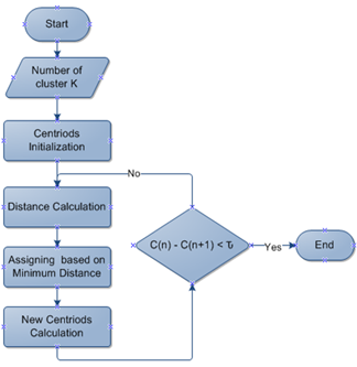
This process is repeated for each data point until the centroid does not change, and there is no difference between c(n) and c(n+1) or the difference is smaller than a threshold value τ is determined by trial, where n is the iteration number. Figure 1 shows the main steps of the K-means clustering algorithm.
Figure 1. K-means algorithm steps
Optimization is the process of finding the optimal solution from all possible solutions in a given space to maximize or minimize its objective function [5]. Gray wolf optimization is a metaheuristic optimization technique identified by Mirjalili [5]. This technique was inspired by the behavior of the grey wolf, its social hierarchy, and its strategy in hunting. Figure 2 depicts the dominant grey wolf social hierarchy, which consists of four categories. The first top one is the leader, who is called the alpha. Alpha has a large amount of authority as it’s responsible for making a decision about the wolves’ lives. The pack should follow the alpha’s decisions and orders. The second level is beta; it helps alpha in decision making and acts as an advisor to it. It should follow the alpha wolves but command the lower level wolves; beta is the best candidate to be alpha. The third level is the delta. Delta wolves have to submit to alphas and betas, but they dominate the omega. Scouts, sentinels, elders, hunters, and caretakers belong to this category. The last ranking wolf is omega; it is the wolves that have to submit to all the other dominant wolves. They are the last wolves that are allowed to eat [5].
Figure 2. Hierarchy of the grey wolf
Hunting strategies are divided into three stages: tracking the prey, encircling it, and attacking it. The mathematical representation of GWO depends on these strategies, $a$ is the best solution, $\beta$ is the second-best solution, and $\delta$ is the thirdbest solution, while $\omega$ wolves follow the upper level [5]. Mathematical models that represent the wolves' behavior in their hunting phases are based on Eqns. (7) and (8) [5].
where, $(X)$ is the position vector of the grey wolf, and $\left(X_p\right)$ is the position vector of prey, $(t)$ is the iteration number, $(C)$ and (A) are coefficient vectors that are calculated based on Eqns. (9) and (10) [5].
where, $\left(r_1\right)$ and $\left(r_2\right)$ are random vectors between 0 and $1,(a)$ is decreased from 2 to 0 .
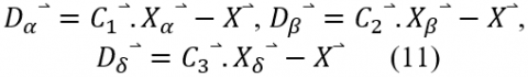
The grey wolves can recognize the prey and encircle it. Also, it updates its positions according to the prey position. It can reach different locations by adjusting the values of (A) and (C). The wolves updated their positions to estimate the prey position based on the wolves a, β, and δ positions shown in Eqns. (11), (12), and (13) [5].
To represent the attack phase by decreasing the random vector (a). (a) is decreased from 2 to 0 over the course of iterations. When random value of A is between -1 and 1, the next position of a search agent can be in any position between its current position and the position of the prey. The attack phase is represented when |A| <1 where the searching for prey phase wolf is represented when |A| >1 which makes GWO searches globally. C is another parameter that must be utilized when modeling the search phase. It contains random values in the interval [0, 2]. It adds weight to prey, making it more difficult for wolves to catch; this affects wolf distance. C is important to show the random behavior of the algorithm and to avoid local optima. It may be considered as the effect of the obstacle. The algorithm searches for the best value of K which is the best position calculated based on the fitness value.
An FPGA is a type of integrated circuit that consists of millions of logic cells that are configured to implement desired algorithms efficiently [16, 17]. The configuration is specified using hardware description languages [18]. FPGAs are widely used in a variety of applications, including industry, military, aerospace, automotive, audio communication, and image processing [18]. The FPGA consists of thousands of fundamental elements named "configurable logic blocks" (CLB). Each CLB consists of several logic blocks which consist mainly of Lookup tables (LUTs), Flip-Flop (FF), Digital Signal Processing (DSP), and others [19].
The FPGA provides a high degree of parallelism in the execution of arithmetic and logical functions. However, the FPGAs require a long time for the design, implementation, and testing processes since the programmer needs to have knowledge of the FPGA architecture [18]. Fortunately, Xilinx FPGA supports a software tool called Vivado HLS [7]. Vivado HLS is an interactive design environment that supports hierarchal design and facilitates the creation and reuse of complex systems. It also accelerates design productivity and enables up to 4X productivity advantages [7]. It includes a built-in simulator that converts C family code into programmable logic [20]. Also, it analyzes all programs in terms of operations, loops, functions, and condition statements. It has many optimization techniques that can be applied to improve the performance in terms of execution time, area, and power dissipation [21].
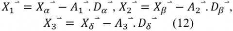
The main objective of this research is to detect the brain tumor by MRI images efficiently by combining the K-means and GWO algorithms. The input image is entered into the GWO algorithm to determine the best number of clusters (K) to segment it as shown in Figure 3. Then, the K-means algorithm starts processing and outputting the clustered image. The methodology includes several steps, starting from searching for the MRI dataset and applying all processing to it until reaching the final outputs, as shown in Figure 3. Figure 4 represents the methodology for all the steps of the proposed algorithm.
Figure 3. Methodology main stages
Figure 4. The proposed methodology flow chart
6.1 Pre-processing
The pre-processing step is needed to prepare the image and enhance its quality [22]. Pre-processing includes the following processes:
6.2 Finding the optimal value of K using Grey Wolf Optimization
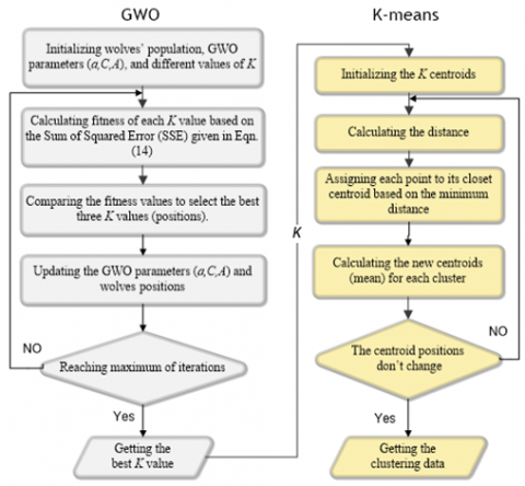
One of the main challenges of the K-mean algorithm is determining the optimal number of clusters to separate the image efficiently [4], which affects the performance of the whole algorithm. In the MRI brain images, it’s very important to choose the correct number of clusters when using K-means clustering to segment the tumor region correctly and separate it from other brain tissues. The grey wolf optimizer (GWO) is used to search and find the optimal value of K where it starts by working on the input image and searching for the best K to segment it by comparing its fitness values as shown in Figure 5. Then, the K value is sent to the K-means algorithm to start the clustering and output of K separate clusters. The steps of the GWO algorithm to find the optimal value of K are as follows:
$f(x)=\sum_{j=1}^k \sum_{i=1}^n\left|b_i-c_j\right|^2$ (14)
where, bi is the intensity of the image pixel, and cj is the centroid of each cluster.
6.3 K-mean clustering
After determining the number of clusters K by GWO, the K-means algorithm starts, and the next step is to initialize the centroid of each cluster. The input image is the dataset that needs to be clustered to assign each pixel to a certain cluster. K centroids are initialized based on Eq. (3). Then, the feature distance between each pixel and each centroid is calculated using Eq. (4) to assign each pixel to its nearest cluster. The next step is to calculate the new mean for all clusters after each iteration. The algorithm is repeated until the mean remains constant or the maximum number of iterations is reached, as shown in Figure 5.
Figure 5. GWO-K-means algorithm flow chart
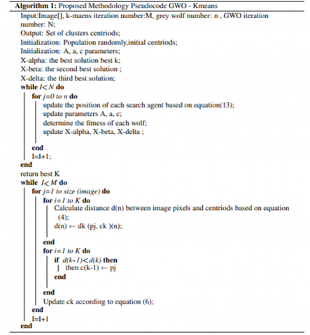
The pseudocode of the proposed GWO-K-means algorithm is shown in Figure 6.
Figure 6. Proposed methodology pseudocode
6.4 Post-processing: Morphological operation
Morphological operations are defined as a technique that deals with the shapes and features of an image [25]. It is used to remove imperfections, and noise after image segmentation, simplify the image, and keep essential shapes. There are two basic types of morphological operations: erosion and dilation [25]. Erosion is used to shrink objects in the images, while dilation is used to grow objects. The combination of erosion and dilation results in two operations: opening and closing [25]. In this research, the K-means algorithm is run on the image to segment it into K clusters. At this step, we can determine to which cluster the tumor belongs. Then, we use the opening operation on the cluster to separate the tumor and remove any noises and imperfections. The opening process is performed by eroding the image with the structuring element and then applying dilation to the eroded image with the same structuring element. The best appropriate structuring element for this type of application, after much experiment testing, was found to be a “disk” (a circle of ones and zeros outside of the circle in the structure element matrix) [26]. The radius of the structure element that was used in this research was 14 pixels [26].
6.5 Optimization on FPGA using Vivado HLS tool
The K-means algorithm is implemented in parallel using an FPGA to improve the performance and reduce the execution time. The parallel implementation allows starting more than one process concurrently. To implement it in parallel on the FPGA, the proposed architecture is replicated according to a parallelization degree. This allows a group of input data to be processed simultaneously. Figure 7 represents the parallel implementation of the K-means algorithm modules. Firstly, the input image is processed row by row in parallel. Each processing unit takes the input image and operates the K-means steps on one row. The input image was replicated N times since each processing element requires its own row and the neighboring rows of the original image to perform some operations and calculations for the distance module, clustering process, and the mean centroid function. The Centroid Register module stores the cluster’s centroids C[m] set which are updated at the end of each iteration. Then, the distance metric module calculates the distances between each data point Pj[m] and each centroid Ck[m].
The clustering process module assigns each data point to its closest cluster. The mean centroid module calculates the new mean of each cluster and stores it on the centroid register. These modules are fully implemented in parallel, so, they are replicated N times based on the hardware resources of the FPGA. This means that an N number of K-means modules are operated concurrently, each one working with a different image row.
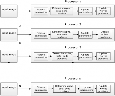
Moreover, the GWO is also implemented on FPGA. The GWO algorithm consists of four iterative modules, which are: the fitness calculation module, determining (alpha, beta, and delta) positions module, updating parameters module, and updating all wolves’ positions module. The input image is replicated N times to enable the simultaneous execution of the module’s function on different rows of the image. As shown in Figure 8, each processing unit takes the input image and works with a different row to operate the GWO algorithm steps in parallel.
The GWO-K-means algorithm was developed using a parallel architecture on FPGA to accelerate the processing time. This is performed by implementing the whole proposed algorithm with the aid of the Vivado HLS tool. Different optimization techniques were adopted and applied, such as loop unrolling, loop pipelining, dataflow, and loop merging. Function pipelining optimization allows processes to run concurrently, whereas loop unrolling allows all loop operations to run in one clock cycle but requires more hardware resources. This helps shorten the execution time.
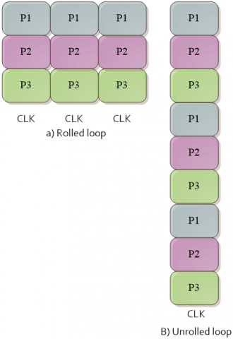
All the initialization steps of the GWO-K-means algorithm don’t have any dependencies, that can be executed in parallel by applying the loop pipelining and loop unrolling as shown in Figures 9 and 10 respectively. Without applying any optimization technique, every iteration needs three clock cycles to operate three processes, which requires 3N clock cycles for N iterations. However, with applying the pipelining optimization technique, only N+2 clock cycles are needed to complete the whole process as shown in Figure 9, and only 1 clock cycle is needed for applying the unrolling optimization technique as shown in Figure 10.
Figure 7. Parallelization of the K-means algorithm
Figure 8. Parallelization of GWO algorithm
Figure 9. Loop pipelining technique
Figure 10. Loop unrolling technique
Figure 11. Data flow technique
The distance and centroids calculations have no dependency, which can be executed in parallel by applying the loop pipelining and loop unrolling optimization techniques. Moreover, it’s not necessary for the update step to wait until the previous step has completely finished all its iterations. Once the current value is determined, it can then be forwarded to the update step to start its execution by applying the dataflow optimization technique as shown in Figure 11. Dataflow is an optimization technique that is applied to the loops to allow parallel execution. Loop 2 can’t start until Loop 1 completes all its iterations. However, while applying the dataflow optimization technique, Loop 1 can forward the result from the first iteration to Loop 2, then both loops can operate concurrently. The same thing between Steps 5 and Step 6 as shown in Figure 11. The Vivado HLS tool automatically inserts channels between the loops to ensure data can flow asynchronously from one loop to the next [27].
Figure 12. GWO-K-means steps and its optimization techniques
Table 1. The results of optimizing the objective function calculation (step 1)
|
|
Before optimization |
After optimization |
|
|
|
Double point |
Fixed point |
|
|
Clock Period (CP) (ns) |
4.36 |
2.39 |
2.39 |
|
Clock Cycles (CC) |
2349954 |
699987 |
100002 |
|
DSP48E |
3 |
2 |
5 |
|
Flip-Flop (FF) |
1128 |
110 |
156 |
|
Lookup Table (LUT) |
880 |
91 |
225 |
|
Execution time (ms) |
10.246 |
1.673 |
0.239 |
|
Speed-up |
1 |
6.124 |
42.87 |
Figure 12 shows all the GWO-K-means steps and the proposed optimization techniques for each step. Step 1 is responsible for determining and calculating the objective function of GWO. It takes the input image and calculates an initial centroid and objective function obj-fun [ ][ ]. The time complexity of this piece of code is O (NM). We applied the pipelining technique to the outer and inner loops since there is no dependency. We also used a fixed-point data type rather than a double point to reduce the resources and the execution time. We used 10 bits for the integer part and 14 bits for the fraction part. After applying the pipelining directive, better results are obtained where there is a notable decrease in the clock cycle, as shown in Table 1. However, there is an increase in FF and LUT, which makes sense because of the parallel execution after pipelining technique that needs more resources. The obtained speed-up of step 1 is 42.87, as shown in Table 1.
Step 2 represents the initialization of the search agent positions, which can be fully parallelized since there is no dependency by applying the loop unrolling and loop pipelining. The obtained speed-up from applying the loop unrolling is 88.7 and 44.71 with applying the pipelining technique as shown in Table 2. More hardware resources are needed for the loop unrolling, so it’s a trade-off issue between the execution time and the usage of hardware resources. However, the processing time for this step is short, and therefore the optimizations for this step were removed since the resources were increased for little improvement in performance. This helps in saving the resources where the bulk of the time is spent.
Table 2. The result of optimization the search agent initialization (step 2)
|
|
Before optimization |
After pipelining |
After unrolling |
|
|
|
Double point |
Fixed point |
|
|
|
Clock Period (CP) (ns) |
3.68 |
2.39 |
2.39 |
2.39 |
|
Clock Cycles (CC) |
2981 |
397 |
103 |
52 |
|
DSP48E |
14 |
10 |
12 |
12 |
|
Flip-Flop (FF) |
3058 |
35 |
31 |
365 |
|
Lookup Table (LUT) |
2235 |
37 |
46 |
1623 |
|
Execution time (ms) |
0.011 |
0.000948 |
0.000246 |
0.000124 |
|
Speed-up |
1 |
11.6 |
44.71 |
88.7 |
Step 3 represents the search agent's fitness value calculation. It was parallelized in the same way using the loop pipelining directive. The obtained speed-up is 618, as shown in Table 3.
Table 3. Result of optimization of the search agent’s fitness value calculation (step 3)
|
|
Before optimization |
After optimization |
|
|
|
Double point |
Fixed point |
|
|
Clock Period (CP) (ns) |
2.49 |
2.39 |
2.39 |
|
Clock Cycles (CC) |
178801 |
149101 |
302 |
|
DSP48E |
0 |
0 |
0 |
|
Flip-Flop (FF) |
36 |
35 |
73 |
|
Lookup Table (LUT) |
48 |
48 |
89 |
|
Execution time (ms) |
0.445 |
0.356 |
0.00072 |
|
Speed-up |
1 |
1.25 |
618 |
Step 4 represents the Alpha, Beta, and Delta wolves' position updating process. Both loop unrolling and pipelining were applied to improve the performance. The obtained speed-up is 6.477, as shown in Table 4.
Table 4. Results of optimizing Alpha, Beta, Delta wolves position updating (step 4)
|
|
Before optimization |
After optimization |
|
|
|
Double point |
Fixed point |
|
|
Clock Period (CP) (ns) |
2.49 |
2.39 |
2.39 |
|
Clock Cycles (CC) |
188650 |
131208 |
30300 |
|
DSP48E |
0 |
0 |
0 |
|
Flip-Flop (FF) |
36 |
35 |
2704 |
|
Lookup Table (LUT) |
48 |
48 |
7061 |
|
Execution time (ms) |
0.469 |
0.313 |
0.0724 |
|
Speed-up |
1 |
1.5 |
6.477 |
Step 5 represents the search agent position updating process. A loop pipelining directive was applied to improve the performance. The obtained speed-up is 32849, as shown in Table 5.
Table 5. Results of optimizing search agent positions updating (step 5)
|
|
Before optimization |
After optimization |
|
|
|
Double point |
Fixed point |
|
|
Clock Period (CP) (ns) |
2.49 |
2.39 |
2.39 |
|
Clock Cycles (CC) |
472290001 |
3030005 |
15006 |
|
DSP48E |
42 |
24 |
31 |
|
Flip-Flop (FF) |
12470 |
88 |
122 |
|
Lookup Table (LUT) |
8901 |
141 |
415 |
|
Execution time (ms) |
1176 |
7.24 |
0.0358 |
|
Speed-up |
1 |
162.43 |
32849 |
Step 6 represents the centroid's initialization. A loop pipelining directive was applied to improve the performance. The obtained speed-up is 9.69, as shown in Table 6.
Table 6. Result of optimizing centroids initialization (step 6)
|
|
Before optimization |
After optimization |
|
|
|
Double point |
Fixed point |
|
|
Clock Period (CP) (ns) |
3.86 |
2.39 |
2.39 |
|
Clock Cycles (CC) |
120001 |
60001 |
20003 |
|
DSP48E |
14 |
10 |
12 |
|
Flip-Flop (FF) |
2579 |
94 |
101 |
|
Lookup Table (LUT) |
2181 |
141 |
162 |
|
Execution time (ms) |
0.4632 |
0.1434 |
0.0478 |
|
Speed-up |
1 |
3.23 |
9.69 |
Step 7 represents the distance matrix calculation. Both loop unrolling and pipelining were applied to improve the performance. The obtained speed-up is 40.377, as shown in Table 7.
Table 7. Result of optimizing the distance matrix calculation (step 7)
|
|
Before optimization |
After optimization |
|
|
|
Double point |
Fixed point |
|
|
Clock Period (CP) (ns) |
3.86 |
2.39 |
2.39 |
|
Clock Cycles (CC) |
50001551 |
18000351 |
2000450 |
|
DSP48E |
3 |
2 |
4 |
|
Flip-Flop (FF) |
871 |
149 |
4104 |
|
Lookup Table (LUT) |
633 |
120 |
9096 |
|
Execution time (ms) |
193 |
43 |
4.78 |
|
Speed-up |
1 |
4.489 |
40.377 |
Table 8. Results of optimizing the minimum distance determining (step 8)
|
|
Before optimization |
After optimization |
|
|
|
Double point |
Fixed point |
|
|
Clock Period (CP) (ns) |
3.86 |
2.39 |
2.39 |
|
Clock Cycles (CC) |
86000101 |
18000101 |
4000500 |
|
DSP48E |
0 |
0 |
0 |
|
Flip-Flop (FF) |
1652 |
181 |
10384 |
|
Lookup Table (LUT) |
1449 |
129 |
11798 |
|
Execution time (ms) |
331.96 |
43.02 |
9.56 |
|
Speed-up |
1 |
7.716 |
34.72 |
Step 8 represents the minimum distance determined. Both loop unrolling and pipelining were applied to improve the performance. The obtained speed-up is 34.72, as shown in Table 8.
Step 9 represents the cluster mean update. Both loop unrolling and pipelining were applied to improve the performance. The obtained speed-up is 35.48, as shown in Table 9.
Table 9. Results of optimizing the clusters means updating (step 9)
|
|
Before optimization |
After optimization |
|
|
|
Double point |
Fixed point |
|
|
Clock Period (CP) (ns) |
4.24 |
2.39 |
2.39 |
|
Clock Cycles (CC) |
100003551 |
21000901 |
5001350 |
|
DSP48E |
12 |
8 |
10 |
|
Flip-Flop (FF) |
20808 |
693 |
28760 |
|
Lookup Table (LUT) |
14253 |
648 |
35284 |
|
Execution time (ms) |
424.02 |
50.2 |
11.95 |
|
Speed-up |
1 |
8.4466 |
35.48 |
The proposed GWO-K-means algorithm has been implemented using MATLAB 2019 on an HP Laptop with an Intel Core i7-6700 GHz running at 3.4 GHz with a memory of 16 GB. For verification purposes to examine the proposed algorithm, MRI image datasets containing T1-weighted and T2-weighted MRI types were used [28]. The grey wolf population is set to 100 search agents, and the iteration number is set to 300. The GWO will return the optimal value of K after completing all the iterations. GWO provides different values of K based on the input image, as shown in Table 10. After clustering, the tumor region will be separated from its cluster using a thresholding technique. Then, a morphological operation was applied to the tumor cluster to enhance the result and remove noise. Table 10 represents a group of MRI images from the dataset and the result after segmenting the brain tumor with different values of K for each image based on GWO.
Several metrics were used to evaluate the performance of the proposed GWO K-means algorithm, including the Silhouette index [29], Mean of Absolute Error MAE [30], Root Mean Square Error RMSE [31], Clusters separation [32], Jaccard index [33], and the Dice index [34]. The Silhouette index measures how similar the point is to points in its own cluster when compared to points in other clusters based on Eq. (15) [24, 29].
$\mathrm{S}_{\mathrm{i}}=\frac{\left(\mathrm{b}_{\mathrm{i}-} \mathrm{a}_{\mathrm{i}}\right)}{\max \left(\mathrm{a}_{\mathrm{i}}, \mathrm{b}_{\mathrm{i}}\right)}$ (15)
where, $a_i$ is the average distance from the ith point to the other points in the same cluster. $b_i$ is the minimum average distance from the ith point to points in a different cluster. The range of silhouette is [-1:1], a value near 1 indicates a correct cluster of the point, whereas a value near -1 indicates a noncorrect cluster of the point.
The MAE measures how closely related points are in the cluster, which is calculated based on Eq. (16) [30].
MAE $=\frac{\sum_{\mathrm{i}=1}^{\mathrm{z}}\left|\mathrm{d}_{\mathrm{i}}-\mathrm{c}\right|}{\mathrm{z}}$ (16)
where, $d_i$ is the data points (the pixel intensity), $c$ is the cluster centroid, and $z$ is the size of the cluster.
The RMSE calculates the error or difference between two values, the lower value is preferred, but it cannot be zero, it indicates the accuracy of the system which is calculated based on Eq. (17) [31].
RMSE $=\sqrt{\frac{1}{Z} * \sum_1^z\left(d_i-c\right)^2}$ (17)
The separation measures how distinct or well separated a cluster is from other clusters, measured by the sum of squares (BSS) between them. The pairwise distance between cluster centers is widely used as a measure of separation, which is calculated based on Eq. (18) [32].
$B S S=\sum_{i=1}^k\left(C-C_i\right)^2$ (18)
Table 10. Results of GWO-K-means for different MRI images
The Jaccard index measures the similarity between two finite sets. It’s defined as the size of the intersections divided by the size of the union of the sample sets A and B, which is calculated based on Eq. (19) [34].
$J(A, B)=\frac{|A \cap B|}{|A \cup B|}$ (19)
The Dice coefficient measures similarity between two sets. It’s very similar to the Jaccard index, which is calculated based on Eq. (20).
$D(A, B)=\frac{2 * J(A, B)}{1+J(A, B)}$ (20)
Table 11. Average silhouette values
|
Image |
Cluster number k |
Average silhouette |
|
1 |
3 |
0.8742 |
|
2 |
5 |
0.8354 |
|
3 |
5 |
0.8127 |
|
4 |
4 |
0.8314 |
|
5 |
4 |
0.9002 |
|
6 |
7 |
0.8589 |
Table 11 represents the silhouette values for the images (1, 2, 3, 4, 5, and 6) in Table (10), respectively. The desirable value of the silhouette index is close to 1. The average silhouette score for image 1 is 0.8742, which is very good and indicates a correct clustering as shown in Table 11. The thickness of the silhouette plot indicates the number of pixels on each cluster; cluster 1 has the largest number of pixels of all the images.
Tables 12, 13, 14, 15, 16, and 17 represent the MAE, RMSE, BSS, Jaccard, and Dice performance metrics for images on Table 10 to evaluate the performance of clustering. The lower MAE and RMSE indicate that the pixels in one cluster are closely related. The pixels in cluster 1 in all images are the closest to each other because of the very low MAE. A high value of BSS means that the clusters are well separated and classified correctly. The Jaccard and Dice indexes represent the similarity between clusters. We want the similarity to be as low as possible to ensure that the pixels on different clusters differ from each other.
Table 18 shows the clustering accuracy for the six images in Table 10, which validates the performance of the proposed algorithm. The same dataset was used for all the tasks to measure the accuracy of classification, which were MRI image datasets containing T1-weighted and T2-weighted MRI types [28].
Table 12. Performance metric for image 1 with K=3
|
Cluster number |
MAE |
RMSE |
BSS |
Jaccard |
Dice |
|
1 |
8.1710*10-20 |
2.8585*10-10 |
4.5362*104 |
0.0145 |
0.286 |
|
2 |
11.9018 |
3.4733 |
1.7438*104 |
0.0034 |
0.0067 |
|
3 |
21.1953 |
4.6863 |
4.0365*104 |
0.0121 |
0.0239 |
Table 13. Performance metric for image 2 with K=5
|
Cluster number |
MAE |
RMSE |
BSS |
Jaccard |
Dice |
|
1 |
5.3473*10-31 |
7.3125*1016 |
1.1570*105 |
0.1887 |
0.3175 |
|
2 |
5.7441 |
2.4010 |
2.3729*104 |
0.0244 |
0.0477 |
|
3 |
6.9528 |
2.6668 |
3.4483*104 |
0.0541 |
0.1026 |
|
4 |
16.2592 |
4.2772 |
4.7408*104 |
0.0089 |
0.0176 |
|
5 |
8.3041 |
2.9245 |
1.0342*105 |
0.0089 |
0.0176 |
Table 14. Performance metric for image 3 with K=5
|
Cluster number |
MAE |
RMSE |
BSS |
Jaccard |
Dice |
|
1 |
3.1343*10-67 |
5.5985*10-34 |
1.2219*105 |
0.0319 |
0.0613 |
|
2 |
9.3186 |
3.0647 |
4.3280*104 |
0.0111 |
0.0219 |
|
3 |
17.4233 |
5.7845 |
3.6683*104 |
0.0595 |
0.1122 |
|
4 |
7.1559 |
2.8467 |
8.5314*104 |
0.0152 |
0.03 |
|
5 |
9.1234 |
3.0825 |
6.2381*104 |
0.0160 |
0.0315 |
Table 15. Performance metric for image 4 with K=4
|
Cluster number |
MAE |
RMSE |
BSS |
Jaccard |
Dice |
|
1 |
1.0718 *10-36 |
2.4723*10-16 |
4.2258*104 |
0.0692 |
0.01294 |
|
2 |
8.4698 |
2.9672 |
1.3601*104 |
0.016 |
0.0315 |
|
3 |
6.1964 |
2.5313 |
1.4747*104 |
0.0541 |
0.1026 |
|
4 |
9.9283 |
4.1668 |
3.5698*104 |
0.0076 |
0.0150 |
Table 16. Performance metric for image 5 with K=4
|
Cluster number |
MAE |
RMSE |
BSS |
Jaccard |
Dice |
|
1 |
5.7065*10-61 |
1.8656*10-18 |
5.8856*104 |
0.0494 |
0.0941 |
|
2 |
6.2113 |
3.0473 |
2.3289*104 |
0.0089 |
0.0176 |
|
3 |
8.7145 |
4.1838 |
2.3472*104 |
0.0252 |
0.0491 |
|
4 |
12.9069 |
4.1345 |
5.8195*104 |
0.0051 |
0.0102 |
Table 17. Performance metric for image 6 with K=7
|
Cluster number |
MAE |
RMSE |
BSS |
Jaccard |
Dice |
|
1 |
4.0509*10-68 |
4.0509*10-68 |
1.3353*105 |
0.1274 |
0.226 |
|
2 |
6.4893 |
7.8065 |
3.196*104 |
0.0516 |
0.0982 |
|
3 |
4.1972 |
4.8435 |
3.7296*104 |
0.3077 |
0.4706 |
|
4 |
4.2863 |
4.99 |
3.3649*104 |
0.0816 |
0.1508 |
|
5 |
7.0793 |
9.0975 |
3.4377*104 |
0.0319 |
0.0618 |
|
6 |
11.3234 |
13.4996 |
69826104 |
0.0149 |
0.0293 |
|
7 |
8.5765 |
9.9967 |
1.1254*105 |
0.016 |
0.0315 |
Table 18. Accuracy of clustering
|
Image |
Cluster number k |
Accuracy |
|
1 |
3 |
94% |
|
2 |
5 |
97.5% |
|
3 |
5 |
98.2% |
|
4 |
4 |
98% |
|
5 |
4 |
96.8% |
|
6 |
7 |
98.2% |
Table 19. Performance metrics for design implementation on both CPU and FPG
|
Performance metrics |
Conventional design on CPU |
Conventional design on FPGA |
Optimized design on FPGA |
|
Execution time (ms) |
2352.43 |
2136.6 |
26.68 |
|
Speed-up |
1 |
1.1 |
88.17 |
Table 20. Time complexity for GWO- K-means algorithm
|
Steps |
Before optimization |
After optimization |
|
Step1: Objective function Calculation |
O(NM) |
O(M) |
|
Step2: Initialization of search agent positions |
O(M) |
O(1) |
|
Step3: Calculation of the fitness values of search agents |
O(NM) |
O(NM)/G |
|
Step4: Updating the positions of wolves Alpha, Beta, Delta |
O(NM) |
O(1) |
|
Step5: Updating positions of each search agent |
O(NM) |
O(NM)/G |
|
Step6: Initializing centroids of k clusters |
O(N+M) |
O(N+M)/G |
|
Step7: Calculation of the distance matrix |
O(NMK) |
O(1) |
|
Step8: Searching for minimum distance to cluster |
O(NMK) |
O(1) |
|
Step9: Updating the clusters mean |
O(NMK) |
O(1) |
|
N is the maximum number of iteration M is the number of search agent’s K is the number of clusters G is the number of defined processing elements |
||
Table 21. Comparison with other research
|
Algorithm |
Speed-up |
Used FPGA device |
|
Reference [35] |
21 |
Xilinx Startix VA7 |
|
Reference [12] |
51.7 |
Xilinx Virtex4 XC4VLX25 |
|
Reference [36] |
20.6 |
Xilinx Kintex-7 |
|
Reference [37] |
30 |
Xilinx XC2V6000 |
|
Proposed method |
88.17 |
Xilinx Kintex7 XC7K160t FPGA 484-1 |
Table 19 shows the performance metrics in terms of execution time and speed-up. The execution time for the conventional design on FPGA is almost the same as for the serial code on CPU (a CPU with an Intel Core i7-6700@3.4 GHz and a memory of 16 GB is used to run the serial code). Compared to implementing the parallel code on FPGA, the execution time was found to be up to 88.17 times slower. This is because the compiler is unable to create pipelined data-paths as a result of the high data dependencies between loops. This is also due to the applied optimization techniques as discussed in the previous section.
The time complexity values for the algorithm steps before and after applying the optimization techniques are represented in Table 20.
Table 21 shows a comparison between the proposed algorithm and other implementations from the related work. It indicates that our algorithm has the best speed-up value among these studies.
A modified GWO-K-means algorithm for earlier and more accurate brain tumor detection by MRI images has been proposed. GWO was adopted to obtain the optimal number of clusters (K) when a large number of search agents are used to search globally for K. The proposed GWO-K-means algorithm was also implemented on FPGA using the Vivado HLS tool to improve the execution time. Different metrics were adopted and applied, such as MAE, RMSE, Silhouette, BSS, Jaccard, and Dice performance metrics, to examine and evaluate the algorithm. The results confirmed a very good clustering of MRI images where the similarity between pixels in one cluster is high and is very low between pixels in different clusters. The average clustering accuracy obtained is 97.11%. Moreover, several optimization techniques such as pipelining, unrolling, and dataflow were adopted and applied to optimize the proposed algorithm on FPGA. This results in a speedup of 88.17 compared to the software sequential-based implementation.
[1] Liu, J., Li, M., Wang, J., Wu, F., Liu, T., Pan, Y. (2014). A survey of MRI-based brain tumor segmentation methods. Tsinghua Science and Technology, 19(6): 578-595. https://doi.org/10.1109/TST.2014.6961028
[2] Martinez, G.V. (2018). Introduction to MRI physics. In Preclinical MRI. Humana Press, New York, NY, pp. 3-19. https://doi.org/10.1007/978-1-4939-7531-0_1
[3] Alam, M.S., Rahman, M.M., Hossain, M.A., Islam, M.K., Ahmed, K.M., Ahmed, K.T., Miah, M.S. (2019). Automatic human brain tumor detection in MRI image using template-based K means and improved fuzzy C means clustering algorithm. Big Data and Cognitive Computing, 3(2): 27. https://doi.org/10.3390/bdcc3020027
[4] Ahmmed, R., Hossain, M.F. (2016). Tumor detection in brain MRI image using template based K-means and Fuzzy C-means clustering algorithm. In 2016 International Conference on Computer Communication and Informatics (ICCCI), pp. 1-6. https://doi.org/10.1109/ICCCI.2016.7479972
[5] Mirjalili, S., Mirjalili, S.M., Lewis, A. (2014). Grey wolf optimizer. Advances in Engineering Software, 69: 46-61. https://doi.org/10.1016/j.advengsoft.2013.12.007
[6] Khatri, A.R., Nizamani, N., Ali, E., Saand, A.S. (2016). Selecting right FPGA for the right application: A technical survey for Xilinx FPGAs. Quaid-E-Awam Univ. Res. J. Eng., Sci. Technol., 15: 46-49.
[7] Xilinx, I. (2013). Introduction to fpga design with vivado high-level synthesis. URL: https://www. xilinx. com/support/documentation/sw_manuals/ug998-vivado-introfpga-design-hls. pdf. (acceso: 28.06. 2020).
[8] Dias, L.A., Ferreira, J.C., Fernandes, M.A. (2020). Parallel implementation of K-means algorithm on FPGA. IEEE Access, 8: 41071-41084. https://doi.org/10.1109/ACCESS.2020.2976900
[9] Hema, M., Madhavi, C. (2014). Tumor Segmentation for Medical Application Using FPGA.
[10] Jaroš, M., Strakoš, P., Karásek, T., Říha, L., Vašatová, A., Jarošová, M., Kozubek, T. (2017). Implementation of K-means segmentation algorithm on Intel Xeon Phi and GPU: Application in medical imaging. Advances in Engineering Software, 103: 21-28. https://doi.org/10.1016/j.advengsoft.2016.05.008
[11] Sotiropoulou, C.L., Gkaitatzis, S., Annovi, A., Beretta, M., Giannetti, P., Kordas, K., Volpi, G. (2014). A multi-core FPGA-based 2D-clustering implementation for real-time image processing. IEEE Transactions on Nuclear Science, 61(6): 3599-3606. https://doi.org/10.1109/TNS.2014.2364183
[12] Hussain, H.M., Benkrid, K., Seker, H., Erdogan, A.T. (2011). FPGA implementation of k-means algorithm for bioinformatics application: An accelerated approach to clustering microarray data. In 2011 NASA/ESA Conference on Adaptive Hardware and Systems (AHS), 248-255. https://doi.org/10.1109/AHS.2011.5963944
[13] Korayem, L., Khorsid, M., Kassem, S.S. (2015). Using grey wolf algorithm to solve the capacitated vehicle routing problem. In IOP Conference Series: Materials Science and Engineering, 83(1): 012014. https://doi.org/10.1088/1757-899X/83/1/012014
[14] Kumar, V., Chhabra, J.K., Kumar, D. (2017). Grey wolf algorithm-based clustering technique. Journal of Intelligent Systems, 26(1): 153-168. https://doi.org/10.1515/jisys-2014-0137
[15] Waleed, M., Um, T.W., Khan, A., Khan, U. (2020). Automatic detection system of olive trees using improved K-means algorithm. Remote Sensing, 12(5): 760. https://doi.org/10.3390/rs12050760
[16] Jarrah, A., Haddad, B., Al-Jarrah, M.A., Obeidat, M.B. (2017). Optimized parallel architecture of evolutionary neural network for mass spectrometry data processing. International Journal of Modeling, Simulation, and Scientific Computing, 8(1): 1750016. https://doi.org/10.1142/S1793962317500167
[17] Alqudah, E., Jarrah, A. (2020). Parallel implementation of genetic algorithm on FPGA using Vivado high level synthesis. International Journal of Bio-Inspired Computation, 15(2): 90-99. https://doi.org/10.1504/IJBIC.2020.106439
[18] Babu, P., Parthasarathy, E. (2021). Reconfigurable FPGA architectures: a survey and applications. Journal of the Institution of Engineers (India): Series B, 102(1): 143-156. https://doi.org/10.1007/s40031-020-00508-y
[19] Jarrah, A., Almomany, A., Alsobeh, A.M., Alqudah, E. (2021). High-performance implementation of wideband coherent signal-subspace (CSS)-Based DOA algorithm on FPGA. Journal of Circuits, Systems and Computers, 30(11): 2150196. https://doi.org/10.1142/S0218126621501966
[20] Jarrah, A., Al-Tamimi, A.K., Albashir, T. (2018). Optimized parallel implementation of extended Kalman filter using FPGA. Journal of Circuits, Systems and Computers, 27(1): 1850009. https://doi.org/10.1142/S0218126618500093
[21] Al Bataineh, A., Jarrah, A., Kaur, D. (2019). High-speed FPGA-based of the particle swarm optimization using HLS tool. International Journal of Advanced Computer Science and Applications, 10(5).
[22] Swiebocka-Wiek, J. (2016). Skull stripping for MRI images using morphological operators. In IFIP International Conference on Computer Information Systems and Industrial Management, 172-182. https://doi.org/10.1007/978-3-319-45378-1_16
[23] Kalvakolanu, A. T. S. (2021). Brain Tumor Detection and Classification from MRI Images.
[24] Ahamad, M.K., Bharti, A.K. (2020). Comparative analysis the fitness function of k-means and kernel fisher’s discriminant analysis (KFDA) with genetic algorithm.'' European Journal of Molecular & Clinical Medicine, 7(11): 6231-6241.
[25] Hÿtch, M., Hawkes, P.W. (2020). Morphological image operators. Academic Press.
[26] Lojzim, J.M., Fries, M. (2017). Brain tumor segmentation using morphological processing and the discrete wavelet transform. Journal of Young Investigators, 33(3). https://doi.org/10.22186/jyi.33.3.55-62
[27] Jarrah, A. (2016). Optimized parallel architecture of Kalman filter for radar tracking applications. Jordan J. Electr. Eng, 2(3): 215-230.
[28] Kawahara, D., Nagata, Y. (2021). T1-weighted and T2-weighted MRI image synthesis with convolutional generative adversarial networks. reports of practical Oncology and radiotherapy, 26(1): 35-42. https://doi.org/10.5603/RPOR.a2021.0005
[29] Mamat, A.R., Mohamed, F.S., Mohamed, M.A., Rawi, N.M., Awang, M.I. (2018). Silhouette index for determining optimal k-means clustering on images in different color models. Int. J. Eng. Technol, 7(2): 105-109.
[30] Kumar, A., Sinha, R., Bhattacherjee, V., Verma, D.S., Singh, S. (2012). Modeling using K-means clustering algorithm. In 2012 1st International Conference on Recent Advances in Information Technology (RAIT), 554-558. https://doi.org/10.1109/RAIT.2012.6194588
[31] Wu, W., Peng, M. (2017). A data mining approach combining K-Means clustering with bagging neural network for short-term wind power forecasting. IEEE Internet of Things Journal, 4(4): 979-986. https://doi.org/10.1109/JIOT.2017.2677578
[32] Liu, Y., Li, Z., Xiong, H., Gao, X., Wu, J. (2010). Understanding of internal clustering validation measures. In 2010 IEEE international conference on data mining, 911-916. https://doi.org/10.1109/ICDM.2010.35
[33] Costa, L.D.F. (2021). Further generalizations of the Jaccard index. arXiv preprint arXiv:2110.09619.
[34] Thada, V., Jaglan, V. (2013). Comparison of jaccard, dice, cosine similarity coefficient to find best fitness value or web retrieved documents using genetic algorithm. International Journal of Innovations in Engineering and Technology, 2(4): 202-205.
[35] Tang, Q.Y., Khalid, M.A. (2016). Acceleration of k-means algorithm using altera SDK for OPENCL. ACM Transactions on Reconfigurable Technology and Systems (TRETS), 10(1): 1-19. https://doi.org/10.1145/2964910
[36] Choi, Y.M., So, H.K.H. (2014). Map-reduce processing of k-means algorithm with FPGA-accelerated computer cluster. In 2014 IEEE 25th International Conference on Application-Specific Systems, Architectures and Processors, 9-16. https://doi.org/10.1109/ASAP.2014.6868624
[37] Saegusa, T., Maruyama, T. (2006). An FPGA implementation of k-means clustering for color images based on KD-tree. In 2006 International Conference on Field Programmable Logic and Applications, 1-6. https://doi.org/10.1109/FPL.2006.311268