Ahmet H. Ornek* | Murat Ceylan
© 2022 IIETA. This article is published by IIETA and is licensed under the CC BY 4.0 license (http://creativecommons.org/licenses/by/4.0/).
OPEN ACCESS
Explaining the decision mechanism of Deep Convolutional Neural Networks (CNNs) is a new and challenging area because of the “Black Box” nature of CNN's. Class Activation Mapping (CAM) as a visual explainable method is used to highlight important regions of input images by using classification gradients. The lack of the current methods is to use all of the filters in the last convolutional layer which causes scattered and unfocused activation mapping. HayCAM as a novel visualization method provides better activation mapping and therefore better localization by using dimension reduction. It has been shown with mask detection use case that input images are fed into the CNN model and bounding boxes are drawn over the generated activation maps (i.e. weakly-supervised object detection) by three different CAM methods. IoU values are obtained as 0.1922 for GradCAM, 0.2472 for GradCAM++, 0.3386 for EigenCAM, and 0.3487 for the proposed HayCAM. The results show that HayCAM achieves the best activation mapping with dimension reduction.
classification, class activation mapping, explainable artificial intelligence, visual explanation, weakly-supervised object detection
In recent years deep learning methods such as Convolutional Neural Networks (CNNs) [1] have found widespread use. Since the CNNs can extract and classify image features automatically, high-performance values for computer vision practices (e.g. image classification, object detection, image segmentation, etc.) have been achieved in medical [2-4], industrial [5-7], agricultural [8-10] and military [11-13] areas.
Although the CNNs achieve high performances, how they decide is not known because a CNN consists of hundreds of non-linear operations and parameters (i.e. CNNs are also known as "Black Box" models) [14]. Explainable Artificial Intelligence (XAI) is a working area aiming at providing numerical, rule-based, and visual explanations to make black box models transparent. Especially visual explanations are commonly used for deep CNNs [15].
The goal of the visual explanation is to highlight the image regions causing the models’ decision (e.g. important regions, object parts, etc.). Class Activation Mapping (CAM) generates activation maps by using convolutions and weights of the CNNs [16]. After CNN made a decision, CAMs highlight the class-related regions over the input images so that end users understand why a decision is made. For instance, if a CNN model classifies a medical image into an "unhealthy" class, CAM aims to highlight the "unhealthy" parts of the medical image.
However, the CAM has limitations in that (i) it does not use fully-connected layers (ii) it is model-dependent (iii) it requires model retraining. To overcome the limitations Gradient-weighted CAM (Grad-CAM) [17] methods have been developed. The Grad-CAM methods are called posthoc methods which means they can be directly applied to the CNNs models without changing any layer after the training and give better explanations than CAMs.
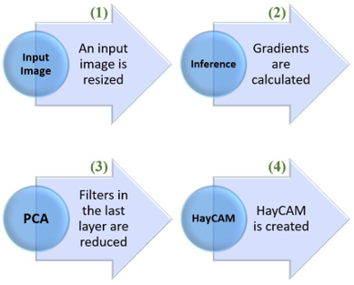
Figure 1. The summarizing of the created HayCAM
HayCAM as a novel visual explanation method for deep CNNs is proposed to give a better activation mapping in this study. The summarizing of the HayCAM can be seen in Figure 1. Figure 1 shows that an input image is resized and fed into the CNN model to get gradients. By using one of the dimension reduction methods that is Principal Component Analysis (PCA), the filters are reduced and HayCAM outputs are obtained.
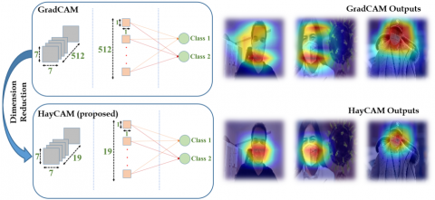
In addition to the explanation sides of the CNNs, better activation mapping brings together better localization that can be used for object detection. By using the activation maps a classifier model is getting the ability to work as an object detector [18-20]. As shown in Figure 2 when 512 filters exist, the GradCAM’s outputs seem to be scattered and unfocused. When dimension reduction is used, 512 filters are reduced to 19 and better activations are obtained.
Figure 2. The illustration of the Haycam. 512 filters cause scattered and unfocused activations maps. Selecting important filters, HayCAM propose better activation mapping
The proposed HayCAM as a novel visual explanation method provides better activation mapping and object detection performance among the other Grad-CAM methods which are Grad-CAM, Grad-CAM++, and Eigen-CAM. Our main contributions are as follows:
The rest of the paper is organized as that the activation mapping works are given in Sec II, the methods having high importance for HayCAM and material are described in Sec III, how the described methods are used together is detailed in Sec IV, and the results are given in the Sec V. The Sec VI and Sec VII show the importance of the achieved results for the proposed HayCAM.
Visualization is one of the most common techniques to make CNN models explainable [21]. Perturbation-based methods observe the prediction changes by windowing the input images with differently shaped regions [22, 23]. Since the windowing operation requires many iteration over the input images, perturbation-based methods’ time cost is bigger than the HayCAM.
LIME creates linear models by changing the input features, and the linear models decide which features affect the classification performance [24]. By not depending on the linear models, SHAP [25] measures the contributions of the features but its computational cost bigger than the LIME. As a rule-based method ANCHORS [26] evaluate all feature space and creates if-then rules so that explanations are obtained. When compared to these methods, HayCAM as a gradient-based method uses non-linear features and does not depend on the if-then rules.
Zeiler et al. [27] propose Deconvolution Networks that extract feature layers from input images by setting a hierarchy. In contrast to HayCAM, it is unsupervised and pixel-space gradient architecture and is not able to produce class-discriminative visualizations.
CAM methods are widely used to generate visual explanations for an input image. The last convolutional layers are weighted by the class-related activations. The first CAM approach [16] uses the last convolutional layer and global average pooling to obtain weighted layers. The drawbacks of this approach are that (i) it does not use fully-connected layers (ii) model-dependent (iii) require model retraining. Since fully-connected layers are not used in the CAM, accuracy does not achieve high values [28].
Since the CAM has limitations, Grad-CAM [17] becomes useful to obtain class-related visual explanations. It does not require any architectural changing or retraining. It uses gradients of desired classes flowing into the last convolution layers to highlight important regions (i.e. it is a class-discriminative method but does not provide fine-grained details). Grad-CAM++ [28] removes the GAP dependency by adding second-order gradients. XCAM [29] scales the gradients by the activations after normalization. ScoreCAM [30] as a posthoc visualization method does not rely on the gradients. It combines the perturbation and CAM-based methods by extracting each activation map with forwarding passes. It brings together the weights and activations linearly. AblationCAM [31] is also a class-discriminative method like Grad-CAM by using ablation analysis. It measures how individual feature maps drop. However, it needs to iterate the gradients many times. LayerCAM [32] uses different layers of CNN architectures and generates activation maps. Although the CAM-based methods can generate the activation maps, they are suffering from using all of the filters in the convolutional layers. HayCAM using dimension reduction removes the unrelated filters to generate better activation mapping.
EigenCAM [33] uncovers the important parts of the input images without modifying the CNN architectures. It computes the important layers by applying Singular Value Decomposition (SVD) and generates smooth activation maps compared to other methods. However, it reduces to one filter which causes losing the importance of related filters. The proposed HayCAM uses principal component analysis as a dimension reduction method and selects the important filters to provide better activation maps.
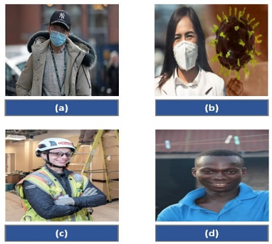
The dataset used for classification has been collected from both open-source and custom images. The details of the collected dataset can be found in “Explainable artificial intelligence: How face masks are detected via deep neural networks” [34] by Ornek et al. The dataset consists of 18400 balanced training images belonging to the "mask" and "no mask" classes. The randomly selected images are shown in Figure 3. When coming to the hardware and software properties used for the practices, can be seen in the Table 1.
Table 1. The used properties for the trainings
|
Programming Language |
Python |
|
Training Environment |
Linux |
|
Deep Learning Framework |
PyTorch |
|
GPU |
Tesla K80 |
|
Images with mask |
9200 |
|
Images without mask |
9200 |
As shown in Table 1 the balanced dataset contains 18400 images with and without mask images. As a programming language Python, deep learning framework PyTorch, and training environment Linux with Tesla K80 GPU have been used.
Figure 3. The randomly selected images from the open-source dataset
3.1 Convolutional Neural Networks (CNNs)
An image classification process can be divided into two categories that are feature extraction and classification. There are traditional feature extraction methods such as histograms of oriented gradients [35] and classification methods such as logistic regression, decision trees, support vector machines, and artificial neural networks [36-39]. Whereas image features are extracted by hand and classified in the traditional methods, these operations are automatically realized by a CNN model [1].
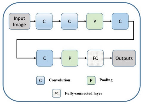
As seen in Figure 4, a CNN model consists of convolutional and fully-connected (FC) layers. The convolutional layer is the combination of convolution (C) and pooling (P) operations that are used for extracting and reducing features, respectively. When an input image is fed into a CNN model, it goes through these layers to get the outputs.
Figure 4. The basic CNN architecture. The convolution (C) and pooling (P) operations are for feature extraction, and the fully-connected (FC) layer is for the classification
Each convolution layer carries different meanings of the given images for example while first convolutions have low-level features such as curve, last convolutions have high-level features such as different parts of the images a.k.a patterns [40]. Image classification, object detection and segmentation problems are solved by using CNN models with high performance values. This model; however, are known as "Black Box" models because millions of non-linear operations and parameters exist in their mechanisms.
3.2 Training the CNN model
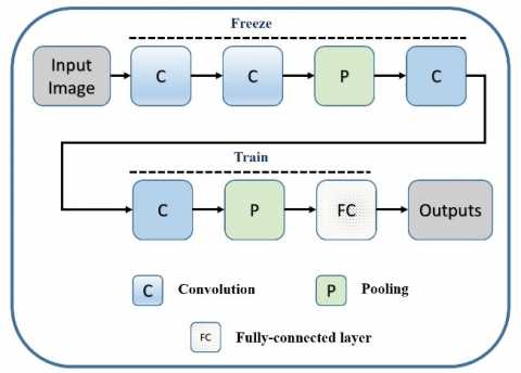
To classify images into "mask" and "no mask" classes transfer learning technique was used in this study. As described in the previous section, when diving into the CNN layers it is seen that while the first layers learn low-level features such as edge, the last layers learn high-level features such as parts of input images. Instead of training the feature extractor part of the CNN model from scratch, a pre-trained model is used as a feature extractor and classifier. Transfer learning can be applied by freezing the first Convolution-Convolution-Pooling-Convolution and training the remaining Convolution-Pooling-Fully connected layers as seen in Figure 5.
Figure 5. The illustration of basic transfer learning. First Convolution-Convolution-Pooling-Convolution are frozen and the remaining Convolution-Pooling-Fully connected layers are trained
Resnet-18 [41] was selected as the pre-trained model that includes 1000 classes belonging to ImageNet [42] dataset. All pre-trained models are always trained with the ImageNet dataset to prove their performance [43-48].
As shown in Figure 5, the first layers of the pre-trained models having low-level features are frozen and only the last layers are trained while the learning process. Since ImageNet has 1000 classes, the changes being at Algorithm 1 should be followed.
As shown at the Algorithm 1 last layer is removed from the pre-trained model and new neurons are added. By freezing the first layers, the model is retrained with the dataset. For the mask classification 2 neurons are added to the pre-trained model as a last layer [49].
Algorithm 1. Transfer learning
Require: X: Pre-trained Model, n: numberof classes
1: X ← remove_last_layer(X)
2: X ← add_new_neurons(n)
3: X ← freeze_first_layers(X)
4: X ← retrain(X)
3.3 Residual Neural Network (Resnet)
When more convolutional layers are used for classification, the product value of the derivatives close to zero and vanishes this issue is known as the vanishing gradient [50]. Achieving more performance requires more convolutional layers; however, as more convolutional layers are used the vanishing gradient problem is seen while the training process.
Resnet is one of the CNN models aiming at providing training without vanishing gradient and makes it possible to train hundreds of layers with high performance [41]. The Resnet uses skip connections to jump over the layers. This layer allows derivatives to be propagated from the last layers to the first layers. 18 layers deep Resnet model known as Resnet18 is shown in Figure 6.
Figure 6. The Resnet18 architecture. (a,b) represents b pieces axa convolution operations (e.g. (3, 64) represents 64 pieces 3x3 convolution operations). The arrows show the skip connections to propagate the derivatives from last layers to first layers
3.4 Gradient-weighted class activation mapping (Grad-Cam)
The CAM method highlights the class-related regions in the input images [16]. The Grad-CAM utilizes the class-related gradients flowing into the last convolutional layer to uncover the important parts of the input images [17]. The last layers of the Resnet-18 can be seen in Figure 7.
Figure 7. The last three layers of the Resnet18. (a) last convolutional layer including 512 pieces 7x7 convolutions. (b) Global Average Pooling that includes 512 pieces 512 pieces 1x1 convolutions. (c) fully-connected layer including two neurons (before the transfer learning there are 1000 neurons)
As shown in Figure 7 (a) Resnet-18 has 512 pieces of 7x7 convolutions in the last convolutional layer. To decrease their size from 7x7 to 1x1 Global Average Pooling (GAP) (1) operation is used in Figure 7 (b). Finally, 2 neurons are used for classification Figure 7 (c).
$G A P=\frac{1}{N} \sum_j \sum_k A_{j k}^h$ (1)
where, Ahjk is the activations of hth layer. By using the GAP operation, the average values of each layer are calculated. In order to get the importance of feature maps whc (GradCAM) is calculated for the hth layer and class c (2).
$w_{h(\text { GradCAM })}^c=\frac{1}{N} \sum_j \sum_k \frac{\partial y^c}{\partial A_{j k}^h}$ (2)
$L_{(\text {GradCAM })}^c=\sum_h w_{h(\text { GradCAM })}^c A^h$ (3)
The gradients of the Yc w.r.t Ah are first computed to achieve the Lc (3) that is the activation (importance) map.
The GAP is applied to the gradients in order to get the wc h (importance weights). The GradCAM process can be summarized as:
When come to the GradCAM++ (4), creating the whc (5) changes.
$L_{(\text {GradCAM }++)}^c=\sum_h w_{h(\text { GradCAM++) }}^c A^h$ (4)
$w_{h(\text { GradCAM }++)}^c=\sum_j \sum_k \alpha_{j k}^{h c} \operatorname{ReLU}\left(\frac{\partial Y^c}{\partial A_{j k}^h}\right)$ (5)
where, αjkhc is pixel-wise weighting values for class c and Ah convolutional layer. The GradCAM++ uses ReLU to ignore the negative gradients (i.e. negative values belonging to other categories) [28]. The sample activation maps (Lcs) are shown in Figure 8.
Figure 8. The randomly selected activation maps
3.5 Principal Component Analyis (PCA)
The dimension reduction methods are used to decrease the feature complexity by selecting prominent features from the feature space (i.e. calculating the feature importance) [51]. PCA is one of the dimension reduction methods. It sorts the features’ importance by measuring the eigenvalues [52]. The PCA algorithm can be seen in Algorithm 2.
According to Algorithm 2, the average value is calculated and subtracted from each value to center the input data. The centered data is used for calculating the covariance matrix. By using the covariance matrix eigenvalues and eigenvectors are calculated so that the input’s features are sorted by the eigenvalues. After the sorting eigenvectors are obtained in descending order and the first n components are selected as important features. The centered data and the selected features are multiplied by the dot product, and reduced data is obtained to be used in the practices. How the PCA is used with Resnet-18 is detailed in Sec IV.
Algorithm 2. PCA
Require: X: input, n: number of components
1: X ← X − mean(X)
2: Cov ← CovarianceMatrix(X)
3: EigenValues ← getvalues(Cov)
4: EigenVectors ← getvectors(Cov)
5: EigenValues ← sort(EigenValues)
6: EigenVectors ← related(EigenValues)
7: EigenVectors ← get(EigenVectors[: n])
8: Output ← X EigenVectors
3.6 Intersection Over Union (IoU)
The object detection models return four values which are x, y, w, and h for a detected object where (x, y) is the top left point’s coordinates, w is width, and h is the height of the bounding box [53] as seen in Figure 9 (a).
The solid line in Figure 9 is called a ground truth bounding box labeled by hand before the training. An object detector tries to properly fit onto the hand-labeled images.
The dashed lines in Figure 9 show the predicted bounding box by the detector.
Figure 9. The bounding box, intersection and union annotations
IoU (6) is used to evaluate the performance of object detection models or object detectors [54]. It calculates how ground truth and predicted bounding boxes are similar by taking intersection and union areas into account. IoU appears between [0, 1], and the values being close to 1 refer to better fitting.
$I o U=\frac{\text { area_of_intersection }}{\text { area_of_union }}$ (6)
This section describes how the methods are used together to create the proposed HayCAM.
HayCAM is a post-pone XAI method like GradCAM which means it can be applied to the CNN models without changing their architectures. In this study Resnet18 architecture is selected as the CNN model and trained with face mask images. The Resnet18 as a pre-trained model has 1000 neurons at the fully-connected layer; however, mask classification requires two neurons to be responsible for the "mask" and "no mask" classes.
To train the Resnet18 with mask images two neurons were placed in the fully-connected layer as shown in Figure 7. The pre-trained model has been trained with 18400 mask images belonging to the "mask" and "no mask" classes as described in Section III-B. The hyper-parameters used for training are as follows; learning_rate: 0.001, momentum: 0.9, loss: cross entropy, epoch: 30, optimizer: stochastic gradient descent.
After the training was completed, the model achieved 96.58% accuracy. But the problem is that it was not known how the model decides that there is a mask in the given image. To make the Resnet18 model transparent GradCAM, GradCAM++, EigenCAM and proposed HayCAM methods have been used so that activation maps will be obtained. The GradCAM as the base method, is detailed at Algorithm 3.
Algorithm 3. GradCAM
Require: X: image
1: X ← resize(X, 224)
2: y ← inference(X)
3: convlayer ← reshape(convlayer)
4: w ← weights(fcl)
5: GradCAM ← w * convlayer
6: GradCAM ← reshape(GradCAM)
7: GradCAM ← resize(GradCAM)
According to Algorithm 3, an input image is resized to 224x224, and the class value is obtained by inference. The last convolutional layer is reshaped from (7x7, 512) to 49x512 and multiplied with the class-related weights between the GAP and the fully-connected layer. To produce the GradCAM, the obtained 1x49 activations are reshaped to 7x7 and then resized to 224x224. The final 224x224 matrix is called as GradCam.
When the activation maps are created by the GradCAM, it is realized that activation maps appear over the mask parts of the given image but they were in a scattered state (the scattered activations can be seen in the following section Figure 12 (a)). The reason is that Resnet18 has 512 convolutions in the last convolutional layer and all of the layers are used to create the final activation map.
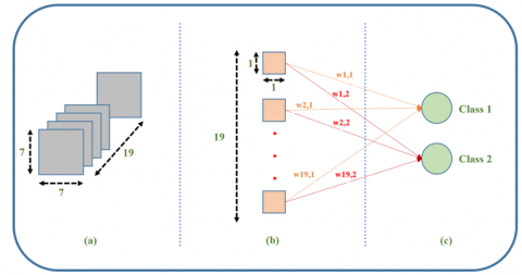
To avoid using all 512 convolutions while creating the final activation map, HayCAM proposed a new method that selects the important convolutions in the last convolutional layer by using a dimension reduction method known as PCA. The proposed HayCAM algorithm is shown in Algorithm 4.
Algorithm 4 resizes the input images to 224x224 and makes an inference to get the class information. The last convolutional layer having 512 pieces of 7x7 convolutions is reshaped to 49x512 and the PCA algorithm is applied to the layer. The first 19 convolutions are selected as having the high-class information, then multiplied with the related weights. The HayCAM is created by reshaping the obtained 1x49 activations to 7x7 and resizing them to 224x224.
The HayCAM structure is shown in Figure 10. By using the HayCAM, convolutions that are less important in view of the classes are reduced so that only main convolutions are used to create the activation maps. HayCAM refers to name of both the method and created activation map.
Algorithm 4. HayCAM (proposed)
Require: X : image, n : number_of_components
1: X ← resize(X, 224)
2: y ← inference(X)
3: convlayer ← reshape(convlayer)
4: convlayer ← convlayer − mean(convlayer)
5: Cov ← CovarianceM atrix(convlayer)
6: EigenValues ← getvalues(Cov)
7: EigenVectors ← getvectors(Cov)
8: EigenValues ← sort(EigenValues)
9: EigenVectors ← related(EigenValues)
10: EigenVectors ← get(EigenVectors[: n])
11: w ← get_related_weights(fcl)
12: HayCAM ← w EigenVectors
13: HayCAM ← reshape(HayCAM)
14: HayCAM ← resize(HayCAM)
Figure 10. The proposed architecture
How experiments are realized and HayCAM is created has been detailed in the previous section. The results section gives the outputs of the experiments which are model performance, visualizing the activation maps, and drawing bounding boxes.
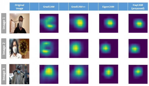
To compare HayCAM with the other methods GradCAM, GradCAM++, and EigenCAM methods are selected. Three test images are used to visualize the obtained results and 160 test images are used to measure the object detection performance. Figure 11 shows the outputs of the Grad-CAM, GradCAM++, EigenCAM, and proposed HayCAM. and Figure 12 shows the combination of input images and outputs of the GradCAM, GradCAM++, EigenCAM, and proposed HayCAM.
After activation maps like those shown in Figure 8 are created four coordinates x, y, w, and h of the bounding boxes are calculated. The obtained images with bounding boxes can be seen in Figure 13.
As described in Sec III-F ground truth bounding boxes are created by hand and object detectors try to find the optimum bounding boxes. IoU is used to measure how predicted bounding boxes are close to ground truths. 160 different images are used to calculate the IoU values for the Grad-CAM, GradCAM++, EigenCAM, and proposed HayCAM. The detailed IoU values are given in Table 2. As seen in Table 2, the proposed HayCAM has the highest average IoU value for the input images.
Figure 11. CAM activation results
Figure 12. CAM results
Table 2. IoU values for all images
|
Image |
GradCAM |
GradCAM++ |
EigenCAM |
HayCAM |
|
|
Image |
1 |
0.1721 |
0.2438 |
0.3246 |
0.3627 |
|
Image |
2 |
0.2128 |
0.3070 |
0.3666 |
0.4822 |
|
Image |
3 |
0.1116 |
0.1463 |
0.1959 |
0.2436 |
|
Image |
4 |
0.2612 |
0.2669 |
0.4425 |
0.5269 |
|
Image |
5 |
0.2291 |
0.3415 |
0.4298 |
0.4420 |
|
Image |
6 |
0.0523 |
0.1214 |
0.1784 |
0.1963 |
|
Image |
7 |
0.0520 |
0.1148 |
0.1701 |
0.1766 |
|
Image |
8 |
0.0499 |
0.1188 |
0.1647 |
0.1829 |
|
Image |
9 |
0.1077 |
0.1651 |
0.2316 |
0.2529 |
|
Image |
10 |
0.0953 |
0.1664 |
0.2404 |
0.2553 |
|
Image |
11 |
0.2501 |
0.3101 |
0.4144 |
0.4483 |
|
... |
|
... |
... |
... |
... |
|
Image |
151 |
0.2259 |
0.2797 |
0.3407 |
0.4381 |
|
Image |
152 |
0.2217 |
0.2832 |
0.3392 |
0.4219 |
|
Image |
153 |
0.1529 |
0.2438 |
0.3397 |
0.4037 |
|
Image |
154 |
0.1486 |
0.1898 |
0.3104 |
0.3676 |
|
Image |
155 |
0.1359 |
0.1856 |
0.2771 |
0.3466 |
|
Image |
156 |
0.1232 |
0.1695 |
0.2972 |
0.3187 |
|
Image |
157 |
0.1205 |
0.1484 |
0.2018 |
0.2115 |
|
Image |
158 |
0.1613 |
0.2226 |
0.3061 |
0.3223 |
|
Image |
159 |
0.1651 |
0.2341 |
0.3021 |
0.3454 |
|
Image |
160 |
0.1486 |
0.1898 |
0.3104 |
0.4277 |
|
Average |
0.1922 |
0.2472 |
0.3386 |
0.3487 |
|
This section discusses the results and shows the importance of the proposed novel HayCAM method. Figure 12 shows that all visualization methods are able to point to which part of the input image is learned by the model. In addition to that the methods’ aim is also provide properly distributed activations for the related class information.
As seen in the Figure 12 while the outputs of the GradCAM are in scattered state, GradCAM++ creates in properly distributed state. The difference between them is that Grad-CAM++ uses second-order and positive gradients.
When come to the outputs of EigenCAM and proposed HayCAM it is seen that the outputs’ distributions are gathered around the class information. EigenCAM uses the SVD technique to reduce the dimension of the last convolutional layer used to create the activation maps; but it directly reduces from 512 convolutions to 1 convolution. This causes losing the class-related information. Instead of reducing from 512 to 1 convolution, HayCAM selects more convolutions having more class information by using the PCA method and reduces convolutions from 512 to 19 convolutions. Therefore, HayCAM provides better activation maps around the class information.
By using the created activation maps object detection is realized by drawing bounding boxes around the high-valued activations. As can be seen in Figure 13, Resnet18 being a classification model can find the objects’ coordinates in the images.
Figure 13. Box detection results IOU values are (b): 0.2061 (c): 0.3062 (d): 0.3714 (e): 0.2061 (f): 0.3714 (h): 0.0875 (i): 0.2973 (j): 0.0875 (k): 0.3604 (l): 0.4635
As described for the activation maps, better-created activations provide better object detection performance that is calculated with IoU. The IoU values can be seen in Table 2. When looking at the average IoU values for 160 images it is seen that GradCAM: 0.1688, GradCAM++: 0.2472, Eigen-CAM: 0.3386, and proposed HayCAM: 0.3487. Whereas the worst IoU is obtained by GradCAM, the best IoU is obtained by the proposed HayCAM method.
The visual explanation methods, aiming at creating activation maps that point to class information, are developed to highlight the class-related parts of the input images. HayCAM as a novel visualization method provides better activation mapping and therefore better localization by using dimension reduction.
The most important limitation of the HayCAM is selecting the number of PCA components. The XAI methods will find more places in the future since just making the right decision is not enough for the end-users and developers. The decision mechanism also should be explained to the experts to build trust in the decisions. We will be continuing to work on XAI, and providing new methods that do not require manually selected parameters such as the number of PCA components with new use cases in the future works.
This study was supported by Huawei Turkey R&D Center.
[1] Krizhevsky, A., Sutskever, I., Hinton, G.E. (2017). Imagenet classification with deep convolutional neural networks. Communications of the ACM, 60(6): 84-90. https://doi.org/10.1145/3065386
[2] Mortazi, A., Bagci, U. (2018). Automatically designing CNN architectures for medical image segmentation. In International Workshop on Machine Learning in Medical Imaging, pp. 98-106. https://doi.org/10.1007/978-3-030-00919-9_12
[3] Zhou, X., Li, Y., Liang, W. (2020). CNN-RNN based intelligent recommendation for online medical pre-diagnosis support. IEEE/ACM Transactions on Computational Biology and Bioinformatics, 18(3): 912-921. https://doi.org/10.1109/TCBB.2020.2994780
[4] Li, Q., Cai, W., Wang, X., Zhou, Y., Feng, D.D., Chen, M. (2014). Medical image classification with convolutional neural network. In 2014 13th International Conference on Control Automation Robotics & Vision (ICARCV), pp. 844-848. https://doi.org/10.1109/ICARCV.2014.7064414
[5] Sharma, P., Jain, S., Gupta, S., Chamola, V. (2021). Role of machine learning and deep learning in securing 5G-driven industrial IoT applications. Ad Hoc Networks, 123: 102685. https://doi.org/10.1016/j.adhoc.2021.102685
[6] Khalil, R.A., Saeed, N., Masood, M., Fard, Y.M., Alouini, M.S., Al-Naffouri, T.Y. (2021). Deep learning in the industrial internet of things: Potentials, challenges, and emerging applications. IEEE Internet of Things Journal, 8(14): 11016-11040. 10.1109/JIOT.2021.3051414
[7] Souza, R.M., Nascimento, E.G., Miranda, U.A., Silva, W. J., Lepikson, H.A. (2021). Deep learning for diagnosis and classification of faults in industrial rotating machinery. Computers & Industrial Engineering, 153: 107060. https://doi.org/10.1016/j.cie.2020.107060
[8] Saleem, M.H., Potgieter, J., Arif, K.M. (2021). Automation in agriculture by machine and deep learning techniques: A review of recent developments. Precision Agriculture, 22(6): 2053-2091. https://doi.org/10.1007/s11119-021-09806-x
[9] Darwin, B., Dharmaraj, P., Prince, S., Popescu, D.E., Hemanth, D.J. (2021). Recognition of bloom/yield in crop images using deep learning models for smart agriculture: A review. Agronomy, 11(4): 646. https://doi.org/10.3390/agronomy11040646
[10] Su, D., Kong, H., Qiao, Y., Sukkarieh, S. (2021). Data augmentation for deep learning based semantic segmentation and crop-weed classification in agricultural robotics. Computers and Electronics in Agriculture, 190: 106418. https://doi.org/10.1016/j.compag.2021.106418
[11] Das, S., Jain, L., Das, A. (2018). Deep learning for military image captioning. In 2018 21st International Conference on Information Fusion (FUSION), pp. 2165-2171. https://doi.org/10.23919/ICIF.2018.8455321
[12] Fernandes, J.D.C.V., de Moura Junior, N.N., de Seixas, J.M. (2022). Deep learning models for passive sonar signal classification of military data. Remote Sensing, 14(11): 2648-2648. https://doi.org/10.3390/rs14112648
[13] Hiippala, T. (2017). Recognizing military vehicles in social media images using deep learning. In 2017 IEEE International Conference on Intelligence and Security Informatics (ISI), pp. 60-65. https://doi.org/10.1109/ISI.2017.8004875
[14] Confalonieri, R., Weyde, T., Besold, T.R., del Prado Martín, F.M. (2021). Using ontologies to enhance human understandability of global post-hoc explanations of black-box models. Artificial Intelligence, 296: 103471. https://doi.org/10.1016/j.artint.2021.103471
[15] Vilone, G., Longo, L. (2020). Explainable artificial intelligence: A systematic review. arXiv preprint arXiv:2006.00093.
[16] Zhou, B., Khosla, A., Lapedriza, A., Oliva, A., Torralba, A. (2016). Learning deep features for discriminative localization. In Proceedings of the IEEE Conference on Computer Vision and Pattern Recognition, pp. 2921-2929. https://doi.org/10.1109/CVPR.2016.319
[17] Selvaraju, R.R., Cogswell, M., Das, A., Vedantam, R., Parikh, D., Batra, D. (2017). Grad-cam: Visual explanations from deep networks via gradient-based localization. In Proceedings of the IEEE International Conference on Computer Vision, pp. 618-626. https://doi.org/10.1109/ICCV.2017.74
[18] Cheng, G., Yang, J., Gao, D., Guo, L., Han, J. (2020). High-quality proposals for weakly supervised object detection. IEEE Transactions on Image Processing, 29: 5794-5804. https://doi.org/10.1109/TIP.2020.2987161
[19] Shao, F., Chen, L., Shao, J., Ji, W., Xiao, S., Ye, L., Zhuang, Y.T., Xiao, J. (2022). Deep learning for weakly-supervised object detection and localization: A survey. Neurocomputing, 496: 192-207. https://doi.org/10.1016/j.neucom.2022.01.095
[20] Dong, B., Huang, Z., Guo, Y., Wang, Q., Niu, Z., Zuo, W. (2021). Boosting weakly supervised object detection via learning bounding box adjusters. In Proceedings of the IEEE/CVF International Conference on Computer Vision, pp. 2876-2885. https://doi.org/10.1109/ICCV48922.2021.00287
[21] van der Velden, B.H., Kuijf, H.J., Gilhuijs, K.G., Viergever, M.A. (2022). Explainable artificial intelligence (XAI) in deep learning-based medical image analysis. Medical Image Analysis, 79: 102470. https://doi.org/10.1016/j.media.2022.102470
[22] Ivanovs, M., Kadikis, R., Ozols, K. (2021). Perturbation-based methods for explaining deep neural networks: A survey. Pattern Recognition Letters, 150: 228-234. https://doi.org/10.1016/j.patrec.2021.06.030
[23] Sudars, K., Namatēvs, I., Ozols, K. (2022). Improving performance of the PRYSTINE traffic sign classification by using a perturbation-based explainability approach. Journal of Imaging, 8(2): 30.. https://doi.org/10.3390/jimaging8020030
[24] Recio-García, J.A., Díaz-Agudo, B., Pino-Castilla, V. (2020). CBR-LIME: A case-based reasoning approach to provide specific local interpretable model-agnostic explanations. In International Conference on Case-Based Reasoning, pp. 179-194. https://doi.org/10.1007/978-3-030-58342-2_12
[25] Fidel, G., Bitton, R., Shabtai, A. (2020). When explainability meets adversarial learning: Detecting adversarial examples using SHAP signatures. In 2020 International Joint Conference on Neural Networks (IJCNN), pp. 1-8. https://doi.org/10.1109/IJCNN48605.2020.9207637
[26] Hase, P., Bansal, M. (2020). Evaluating explainable AI: Which algorithmic explanations help users predict model behavior? arXiv preprint arXiv:2005.01831.
[27] Zeiler, M.D., Krishnan, D., Taylor, G.W., Fergus, R. (2010). Deconvolutional networks. In 2010 IEEE Computer Society Conference on computer vision and pattern recognition, pp. 2528-2535. https://doi.org/10.1109/CVPR.2010.5539957
[28] Chattopadhay, A., Sarkar, A., Howlader, P., Balasubramanian, V.N. (2018). Grad-CAM++: Generalized gradient-based visual explanations for deep convolutional networks. In 2018 IEEE winter conference on applications of computer vision (WACV), pp. 839-847. https://doi.org/10.1109/WACV.2018.00097
[29] Fu, R., Hu, Q., Dong, X., Guo, Y., Gao, Y., Li, B. (2020). Axiom-based grad-cam: Towards accurate visualization and explanation of CNNs. arXiv preprint arXiv:2008.02312.
[30] Wang, H., Wang, Z., Du, M., et al. (2020). Score-CAM: Score-weighted visual explanations for convolutional neural networks. In Proceedings of the IEEE/CVF Conference on Computer Vision and Pattern Recognition Workshops, pp. 24-25. https://doi.org/10.1109/CVPRW50498.2020.00020
[31] Ramaswamy, H.G. (2020). Ablation-CAM: Visual explanations for deep convolutional network via gradient-free localization. In Proceedings of the IEEE/CVF Winter Conference on Applications of Computer Vision, pp. 983-991. https://doi.org/10.1109/WACV45572.2020.9093360
[32] Jiang, P.T., Zhang, C.B., Hou, Q., Cheng, M.M., Wei, Y. (2021). LayerCAM: Exploring hierarchical class activation maps for localization. IEEE Transactions on Image Processing, 30: 5875-5888. https://doi.org/10.1109/TIP.2021.3089943
[33] Muhammad, M.B., Yeasin, M. (2020). Eigen-cam: Class activation map using principal components. In 2020 International Joint Conference on Neural Networks (IJCNN), pp. 1-7. https://doi.org/10.1109/IJCNN48605.2020.9206626
[34] Ornek, A.H., Celik, M., Ceylan, M. (2021). Explainable artificial intelligence: How face masks are detected via deep neural networks. International Journal of Innovative Science and Research Technology, 6(9): 1104-1112.
[35] Rybski, P.E., Huber, D., Morris, D.D., Hoffman, R. (2010). Visual classification of coarse vehicle orientation using histogram of oriented gradients features. In 2010 IEEE Intelligent Vehicles Symposium, pp. 921-928. https://doi.org/10.1109/IVS.2010.5547996
[36] Ullah, S.I., Salam, A., Ullah, W., Imad, M. (2021). COVID-19 lung image classification based on logistic regression and support vector machine. In European, Asian, Middle Eastern, North African Conference on Management & Information Systems, pp. 13-23. https://doi.org/10.1007/978-3-030-77246-8_2
[37] Chandra, M.A., Bedi, S.S. (2021). Survey on SVM and their application in image classification. International Journal of Information Technology, 13(5): 1-11. https://doi.org/10.1007/s41870-017-0080-1
[38] Pastorino, M., Montaldo, A., Fronda, L., Hedhli, I., Moser, G., Serpico, S.B., Zerubia, J. (2021). Multisensor and multiresolution remote sensing image classification through a causal hierarchical Markov framework and decision tree ensembles. Remote Sensing, 13(5): 849-849. https://doi.org/10.3390/rs13050849
[39] Kumar, K.K., Kumar, M.D., Samsonu, C., Krishna, K.V. (2021). Role of convolutional neural networks for any real time image classification, recognition and analysis. Materials Today: Proceedings. https://doi.org/10.1016/j.matpr.2021.02.186
[40] Albawi, S., Mohammed, T.A., Al-Zawi, S. (2017). Understanding of a convolutional neural network. In 2017 International Conference on Engineering and Technology (ICET), pp. 1-6. https://doi.org/10.1109/ICEngTechnol.2017.8308186
[41] He, K., Zhang, X., Ren, S., Sun, J. (2016). Deep residual learning for image recognition. In Proceedings of the IEEE Conference on Computer Vision and Pattern Recognition, pp. 770-778. https://doi.org/10.1109/CVPR.2016.90
[42] Russakovsky, O., Deng, J., Su, H., et al. (2015). ImageNet large scale visual recognition challenge. International journal of computer vision, 115(3): 211-252. https://doi.org/10.1007/s11263-015-0816-y
[43] Iandola, F., Moskewicz, M., Karayev, S., Girshick, R., Darrell, T., Keutzer, K. (2014). Densenet: Implementing efficient convnet descriptor pyramids. arXiv preprint arXiv:1404.1869.
[44] Szegedy, C., Ioffe, S., Vanhoucke, V., Alemi, A.A. (2017). Inception-v4, inception-ResNet and the impact of residual connections on learning. In Thirty-first AAAI Conference on Artificial Intelligence.
[45] Kornblith, S., Shlens, J., Le, Q.V. (2019). Do better ImageNet models transfer better? In Proceedings of the IEEE/CVF Conference on Computer Vision and Pattern Recognition, pp. 2661-2671. https://doi.org/10.1109/CVPR.2019.00277
[46] Zoph, B., Vasudevan, V., Shlens, J., Le, Q.V. (2018). Learning transferable architectures for scalable image recognition. In Proceedings of the IEEE Conference on Computer Vision and Pattern Recognition, pp. 8697-8710. https://doi.org/1109/CVPR.2018.00907
[47] Simonyan, K., Zisserman, A. (2014). Very deep convolutional networks for large-scale image recognition. arXiv preprint arXiv:1409.1556.
[48] Chollet, F. (2017). Xception: Deep learning with depthwise separable convolutions. In Proceedings of the IEEE Conference on Computer Vision and Pattern Recognition, pp. 1251-1258. https://doi.org/10.1109/CVPR.2017.195
[49] Ornek, A.H., Ceylan, M. (2021). Explainable artificial intelligence (XAI): Classification of medical thermal images of neonates using class activation maps. Traitement du Signal, 38(5): 1271-1279. https://doi.org/10.18280/ts.380502
[50] Liu, M., Chen, L., Du, X., Jin, L., Shang, M. (2021). Activated gradients for deep neural networks. IEEE Transactions on Neural Networks and Learning Systems, pp. 1-13. https://doi.org/10.1109/TNNLS.2021.3106044
[51] Kherif, F., Latypova, A. (2020). Principal component analysis. In Machine Learning, pp. 209-225. https://doi.org/10.1016/B978-0-12-815739-8.00012-2
[52] Wu, S. X., Wai, H.T., Li, L., Scaglione, A. (2018). A review of distributed algorithms for principal component analysis. Proceedings of the IEEE, 106(8): 1321-1340. https://doi.org/10.1109/JPROC.2018.2846568
[53] Zhao, Z.Q., Zheng, P., Xu, S.T., Wu, X. (2019). Object detection with deep learning: A review. IEEE transactions on neural networks and learning systems, 30(11): 3212-3232.. 10.1109/TNNLS.2018.2876865
[54] Zhou, D., Fang, J., Song, X., Guan, C., Yin, J., Dai, Y., Yang, R. (2019). IoU loss for 2D/3D object detection. In 2019 International Conference on 3D Vision (3DV), pp. 85-94. https://doi.org/10.1109/3DV.2019.00019