Li Duan | Jianxian Cai* | Juan Liang | Danqi Chen | Xiaoye Sun
© 2022 IIETA. This article is published by IIETA and is licensed under the CC BY 4.0 license (http://creativecommons.org/licenses/by/4.0/).
OPEN ACCESS
Deep learning is not the most accurate way for recognizing time series signals, and it is unable to identify non-stationary time series signals with numerous chaotic classes. Moreover, the signal detection benefits from data preprocessing have gone unnoticed. Therefore, this paper investigates the detection and analysis of non-stationary time series signals using deep learning and data preprocessing. The fitting model of the historical stationarity index is built based on the Gaussian mixture model of single Gaussian models, and the change point of the non-stationary time series signal is detected. To further increase the signal's recognition rate, the non-stationary time series signal is preprocessed using the truncated migration algorithm. The main classification task and the auxiliary classification tasks are constructed to identify non-stationary time series signals characterized by huge chaotic classes through multi-task learning. The efficiency of the suggested method and model is validated by experimental data.
data preprocessing, deep learning, non-stationary time series signal, signal recognition
Time series signals can illustrate how things or phenomena change over time in terms of their state or intensity. This energizes ongoing studies into these signals [1-6]. One of the key study areas is the identification and analysis of non-stationary time series signals, which has been applied in a variety of industries and fields, including streaming media, meteorology, medicine, and business [7-17]. Researchers both domestically and internationally have been using deep learning techniques with significant self-learning capabilities to detect time series signals in recent years, but the signal recognition rate is still suboptimal [18-23]. With change point monitoring as a representative application scenario, the extraction of time series signal stationarity indicators and the development of deep learning techniques to enhance signal recognition accuracy represent an unavoidable trend and have significant practical implications.
It is well known that research has been done on non-stationary acoustic signal filtering techniques based on wavelet threshold denoising. This method calls for the usage of a significant amount of CPU resources for processing huge volumes of data. A different method for building CF based on the McCulloch-Pitts neuron model was proposed by Khobotov et al. [24]. This neuron-like CF relies exclusively on logical processes, which employ fewer CPU resources, and is based on particular nonlinear transformations of input and test signals. The results are thought to be applicable to a wide range of real-world scenarios involving long-range sonar, seafloor detection, and non-stationary environments. Empirical Fourier Decomposition (EFD), a method that combines the improved Fourier spectral segmentation methodology and the usage of zero-phase filter banks, was proposed by Zhou et al. [25] as a precise adaptive signal decomposition tool. A numerical analysis was done to look at the reliability and accuracy of EFD. The results demonstrate that for signals with several non-stationary modes and closely spaced modes, EFD can yield accurate and reliable decomposition results. Ding et al. [26] created the Kernel Ridge Regression-based Chirp Transform (KRR-CT) to precisely identify the TF features of non-stationary signals and build energy-concentrated TF flats since the solution of the polynomial approximation is easily influenced by noise or interference. Even with significant noise present, a stable solution can be produced in the KRR-CT approximation stage. Wang et al. [27] addressed a number of frequently employed time-frequency analysis techniques for non-stationary signals, examined these techniques with mixed signals and noise, and then went into great depth into the benefits and drawbacks of each technique. The study of the time-frequency of the continuous wave radio Doppler signal produced when the missile strikes the target using an enhanced time-frequency analysis approach based on STFT is proposed. The aforementioned technique is used to process real experimental data, and positive results are obtained. This validates that the method is feasible and effective, and will significantly support any further information processing or calculation.
Research on various non-stationary signal identification and analysis techniques based on signal processing theory has been extensive both domestically and internationally. While neglecting the positive impact of data preprocessing on signal identification, there is currently no solution that can address the issue of recognizing non-stationary time series signals of vast chaotic classes. Therefore, this work investigates the detection and analysis of non-stationary time series signals using deep learning and data preprocessing. Chapter 2 completes the identification of the change point of the non-stationary time series signal and builds the fitting model of the historical stationarity index based on the Gaussian mixture model of single Gaussian models. To further increase the signal's recognition rate, the non-stationary time series signal is preprocessed in Chapter 3 using the truncated migration algorithm. The main classification goal and an auxiliary classification assignment are designed in Chapter 4 to identify non-stationary time series signals characterized by vast chaotic classes. The efficiency of the suggested method and model is validated by experimental data.
Time series signal stationarity can be dynamically defined via stationarity indicators. The amplitude of the stationarity index will quickly grow or drop for non-stationary time series signals as the signal transitions from a stationary to a non-stationary state. It is evident that the change in the condition of the time series signal occurs at the same time as the stationarity index begins to fluctuate. It is required to find the non-stationary time series signal's transition point before recognizing the non-stationary time series signal itself.
Building a fitting model of the historical stationarity index first, then determining if the present stationarity index complies with the model, is the typical method for detecting changes in the stationarity index. The historical stationarity index fitting model in this study is built using the Gaussian mixture model of single Gaussian models. The probability distribution formula for the single Gaussian model is given by the expression ω=(r*, ε2), where r* and ε are the mean and standard deviation of the estimated Gaussian distribution, respectively:
$h(r \mid \omega)=\frac{1}{\sqrt{2 \pi \varepsilon^2}} \exp \left(-\frac{\left(r-r^*\right)^2}{2 \varepsilon^2}\right)$ (1)
r* and ε can be respectively calculated by:
$r^*=\frac{1}{m} \sum_{j=1}^m r_j$ (2)
$\varepsilon=\sqrt{\frac{1}{m} \sum_{j=1}^m\left(r_j-r^*\right)^2}$ (3)
Let βh be the mixture coefficient of each Gaussian model, and βh≥0, ∑Hh=1 βh=1. The probability distribution of the Gaussian mixture model composed of h single Gaussian models can be expressed as:
$h(r \mid \omega)=\sum_h^H=1 \beta_h \psi\left(r \mid \omega_h\right)$ (4)
The distribution density ψ(r|ωh) of the h-th Gaussian model can be given by:
$\psi\left(r \mid \omega_h\right)=\frac{1}{\sqrt{2 \pi \varepsilon_h^2}} \exp \left(-\frac{\left(r-r_h^*\right)^2}{2 \varepsilon_h^2}\right)$ (5)
Let ωh=(rh*,ε2h) be the h-th Gaussian model, whose mean and standard deviation are similar to Eq. (2) and Eq. (3), respectively. Then, the Beta distribution is defined in the (0, 1) interval. Assume that the hyperparameters of the Beta distribution are represented by β and γ, and the Beta function is represented by Y(β, γ). The probability distribution of the Beta distribution can be expressed as:
$h(r \mid \beta, \gamma)=\frac{1}{Y(\beta, \gamma)} r^{\beta-1}(1-r)^{\omega-1}$ (6)
The Beta function Y(β, γ) can be expressed as:
$Y(\beta, \gamma)=\int_0^1 b^{\beta-1}(1-b)^{\gamma-1} d b$ (7)
The single Gaussian model constructed in this way is suitable for any random time series signal data. ITo detect whether the abnormality of the time series signal occurs at the (m+1)-th time, this paper conducts a hypothesis test on the model based on the PauTa criterion. Assuming that |rm+1-rm*|<lε is satisfied, then the time series signal state does not change at the (m+1)-th moment, represented by F0; when |rm+1-rm*| ≥lε, the signal state changes, denoted by F1, means that the following process:
$F_0:\left|r_{m+1}-\bar{r}_m\right|<l \varepsilon$
$F_1:\left|r_{n+1}-\bar{r}_n\right| \geq l \varepsilon$ (8)
The traditional signal recognition model usually has the problem of a limited receptive field, which makes the extracted signal timing features not objective enough. To further improve the recognition rate of non-stationary time series signals, this paper uses the truncated migration algorithm to preprocess the signals, and constructs a new sampling matrix, which enables the signal recognition model to extract more sampling points and signal symbols. Figure 1 shows the processing flow of the non-stationary time series signals.
The information features of non-stationary time series signals can be generated by fusing the space and channel information in the local receptive field. Suppose the convolution operation is represented by ⊗, the input is represented by A, the feature is represented by G, the convolution kernel is represented by L, L$\in$Rl×l, the size of the convolution kernel is represented by l. Then, the convolutional operation can be expressed as:
$G=A \otimes L$ (9)
The receptive field of G is limited by L and A. Changes in the sign of a signal are characteristic for non-stationary time series signal identification. Traditional signal recognition models are difficult to capture long-term dependencies, and can only classify non-stationary time series signals by comparing the signal signs of each sampling point. In this paper, the data truncation migration algorithm is used to enable the signal recognition model to compare more symbolic information. The specific steps of the algorithm are as follows:
Step 1: Assuming that the length is represented by k, and the width and channel dimensions are 2 and 1, respectively. Then, the sampling matrix BC can be reshaped as (2, k, 1).
Step 2: Set the distance R to be moved to describe a truncation and the number of truncation movement times BP.
Step 3. Let B0 be the original sampling matrix i. Migrate the 1×R truncation at the right end of B0 to the leftmost of that matrix to produce matrix B1. Then migrate the 2×R truncation at the right end of B1 to the leftmost of B1 to produce matrix B2. Perform similar migration P times to produce matrix BP.
The combination of B0 and B1 makes {bk}, kÎ[1, R] close to {bk}, kÎ[k-R+1, k} in the horizontal direction, and close to {bk}, kÎ[R, 2R] in the vertical direction. The combination of B1 and B2 makes {bk}kÎ[R, 3R] close to {bk}, kÎ[1, R] and {bk}, kÎ[k-R-1, k} in the horizontal direction, and close to {bk}, kÎ[3R, 5R] in the vertical direction, and so on.
Step 4. After moving P times, if the following formula is established, return to Step 3. Otherwise, go to Step 5.
$\frac{P \times(P+1) \times R}{2}<k$ (10)
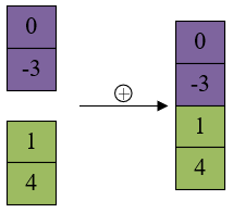
Step 5: Merge the sampling matrices B0 to BP through the "Concatenate" operation (Figure 2), and denote the generated new sampling matrix by BIW. The size of BIW is (2P+2, k, 1), and the "Concatenate" operation is represented by "⊕". Then, BIW can be formed by the following formula:
$B_{I W}=B_0 \oplus B_1 \oplus \ldots \oplus B_P$ (11)
Step 6: Convert BIW into a sampling matrix BXT based on amplitude X and phase T:
$X=\sqrt{I^2+W^2}$
$T=\arctan (I / W)$ (12)
Step 7: Merge BIW and BXT in the channel dimension through feature concatenation. Take the formed new matrix as the input of the classifier B'C, then:
$B_C^{\prime}=B_{I W} \oplus B_{X T}$ (13)
To enhance the extracted non-stationary time series signal features, the conversion result of the sampling matrix is transformed into the form of polar coordinates through Steps 6 and 7. The final output is matrix B'C of the size (2P+2, k, 2).
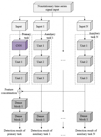
Figure 1. Processing flow of the non-stationary time series signal
Figure 2. Operation principle of feature concatenation
Confusion can easily result from non-stationary time series signals whose distribution law is time-dependent. In order to recognize non-stationary time series signals defined by significant chaotic classes, this paper introduces multi-task learning. In this study, the network that can discriminate between two non-stationary time series signals is employed for auxiliary classification tasks, with the multi-task learning network's primary task being the identification of all non-stationary time series signals. On this basis, this paper connects gated recurrent unit (GRU), responsible for the auxiliary tasks, with convolutional neural network (CNN), responsible for the primary task, in series into a model (Figure 3).
The GRU model contains two gates, the update gate cp and the reset gate sp. The state fp at time p depends on how much information is inherited from state fp-1 at time p-1, and how much new information is extracted from the candidate state ḟp at time p. Both of the information volumes are decided by the update gate cp. The value of cp increases with the importance of the state at the previous moment to the state at the current moment. Let ap be the input vector at the current moment, Qc be the weight matrix of the update gate, ε(.) be the sigmoid function, and yc be the bias of the update gate. Then, cp can be calculated by:
$c_p=\varepsilon\left(Q_c a_p+Q_c f_{p-1}+y_c\right)$ (14)
Whether the candidate state ḟp at time p depends on the state fp-1 at time p-1 depends on the reset gate sp. The less important the state at the previous moment to the state at the current moment, the smaller the sp. Let Qs and ys be the weight and bias of the reset gate, respectively. Then, sp can be calculated by:
$s_p=\varepsilon\left(Q_s a_p+Q_s f_{p-1}+y_s\right)$ (15)
Let Qf, yf and ○ be weight, bias, and Hadamard product, respectively. Then, the candidate state ḟp can be calculated by:
$\dot{f}_p=\operatorname{Tanh}\left(Q_f a_p+Q_f\left(s_p \circ f_{p-1}\right)+y_f\right)$ (16)
The output of the GRU model can be expressed as:
$f_p=\left(1-c_p\right) \circ f_{p-1}+c_p \circ \dot{f}_p$ (17)
Since this article sets up several auxiliary task models for the non-stationary time series signal identification model, it is vital to thoroughly analyze the over-fitting phenomenon of the model, even though the performance of the GRU model will improve as the number of layers grows. In this study, a 3-layer GRU model is constructed.
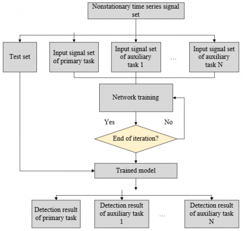
The primary classification job model for non-stationary time series signals accepts input in the one-dimensional time series A/P format. In order to increase the rate at which non-stationary time series signals are recognized, this study builds a model for the primary task classification using CNN and GRU in series. It also realizes the merging of the spatial and temporal aspects of the signal. The model training process is shown in Figure 4.
Figure 3. Structure of the detection model
Figure 4. Flow of model training
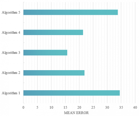
The results of data preprocessing using various numbers of single Gaussian models are shown in Figure 5. The algorithms in this work correspond to algorithms 1 through 5, with 2, 3, 4, 5, and 6 being the number of single Gaussian models, respectively. The figure shows that the error value of the non-stationary time series signal change point detection is lowest when the number of single Gaussian models is 4. Thus, it is determined that there should be exactly four single Gaussian models.
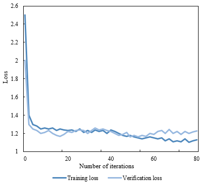
Figure 6 displays the recognition model's training and validation losses. The figure shows that the model's convergence occurs quickly, there is no over-fitting after 80 iterations, and both the training set's and the test set's performance are satisfactory. Table 1 displays, for various values of the distance R to be shifted by a truncation, the accuracy of non-stationary time series signal detection. The average value and maximum value of the non-stationary time series signal recognition rate are at their highest when the distance to be moved for a truncation is 4. Currently, less than 1 second is needed for one iteration, which is also within the allowed range of less than 1 minute.
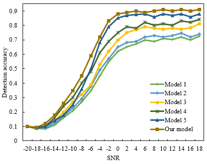
Figure 7 compares the detection accuracies of different signal recognition models. It is observed that, with the growth of the signal to noise ratio (SNR), the signal recognition effect of five detection models all improves, including the envelope feature-based model, the double spectra feature-based model, the wavelet transform feature-based model, the multilayer perceptron (MLP), and long short-term memory (LSTM) model. The envelope feature-based model, the double spectra feature-based model, the wavelet transform feature-based model cannot extract more time series features of nonstationary time series signals, or fuse the spatial and temporal features of the signals. Their highest detection accuracy is around 70%. Despite capable of extracting spatial and temporal features, the MLP cannot connect adjacent time domain signals, and its accuracy is about 80%. Our model fuses the spatial and temporal features of the signals, and differentiates the signals with confusion phenomenon. The highest accuracy is around 90%.
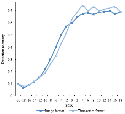
The detection accuracies with different input formats were compared to further verify the effectiveness of our model on nonstationary time series signals. As shown in Table 2 and Figure 8, the detection accuracies with the two formats (image format and time series format) are similar. It is verified that the one-dimensional time-series format input, which has certain advantages in theory, also has ideal recognition performance in the actual process of signal recognition with confusion. Compared with the other five models, our model boasts high mean accuracies with both two input formats. Whether the SNR is low, medium or high, our model can recognize nonstationary time series signals better than the image format. This further verifies the effectiveness of our model.
Table 1. Detection accuracies at different R values
|
R |
Maximum accuracy |
Mean accuracy |
Matrix shape |
Iterative time |
|
1 |
95.27% |
63.58% |
(36,114,6) |
142s |
|
2 |
93.24% |
67.42% |
(25,174,1) |
85s |
|
3 |
93.52% |
69.18% |
(11,196,5) |
61s |
|
4 |
98.31% |
70.54% |
(18,142,1) |
59s |
|
5 |
96.47% |
66.37% |
(16,195,4) |
51s |
|
6 |
94.18% |
51.24% |
(13,127,6) |
57s |
Figure 5. Change point detection errors of different signal Gaussian models
Figure 6. Training and verification losses of the identification model
Figure 7. Detection accuracies of different signal recognition models
Figure 8. Detection accuracies of input formats
Table 2. Mean detection accuracies with different input formats
|
Model number |
Input format |
Mean detection accuracy |
|||
|
SNR interval |
Low SNR |
Medium SNR |
High SNR |
||
|
1 |
Image |
62.14 |
21.62 |
50.81 |
80.92 |
|
Time series |
59.82 |
19.85 |
59.27 |
84.26 |
|
|
2 |
Image |
52.65 |
17.34 |
50.61 |
68.04 |
|
Time series |
44.96 |
18.51 |
42.78 |
76.92 |
|
|
3 |
Image |
59.81 |
19.14 |
63.61 |
85.37 |
|
Time series |
63.47 |
19.39 |
57.41 |
80.69 |
|
|
4 |
Image |
65.23 |
27.52 |
60.81 |
88.92 |
|
Time series |
64.58 |
20.45 |
61.21 |
89.24 |
|
|
5 |
Image |
72.68 |
21.04 |
68.61 |
88.09 |
|
Time series |
81.49 |
24.91 |
70.74 |
89.96 |
|
|
Our model |
Image |
80.47 |
29.34 |
73.69 |
91.32 |
|
Time series |
89.22 |
31.76 |
77.61 |
95.62 |
|
This paper investigates the detection and analysis of non-stationary time series signals using deep learning and data preprocessing. The fitting model of the historical stationarity index is built based on the Gaussian mixture model of single Gaussian models, and the change point of the non-stationary time series signal is detected. To further increase the signal's recognition rate, the non-stationary time series signal is preprocessed using the truncated migration algorithm. The main classification task and the auxiliary classification tasks are constructed, and coupled with multi-task learning, to identify non-stationary time series signals characterized by huge chaotic classes through multi-task learning. Through experiments, the change point detection errors of different number of single Gaussian models are compared, indicating that the best number is 4. Then, the training and validation looses of the recognition model were presented, which confirm that the model converges quickly. In addition, the detection accuracies at different R values and of different models were contrasted. The results show that the one-dimensional time-series format input, which has certain advantages in theory, also has ideal recognition performance in the actual process of signal recognition with confusion. Finally, the mean recognition accuracies of models with different input formats are compared, suggesting the effectiveness of our algorithm and model.
This work was supported by the Fundamental Research Funds for the Central Universities (Grant No.: ZY20215214); Langfang Science and Technology Research Self-Funded Project (Grant No.: 2022011012); Fundamental Research Funds for the Central Universities (Grant No.: ZY20215217). The research work of this paper is performed at the Hebei Key Laboratory of Seismic Disaster Instrument and Monitoring Technology.
[1] You, Y.H., Song, H.K. (2020). Efficient sequential detection of carrier frequency offset and primary synchronization signal for 5G NR systems. IEEE Transactions on Vehicular Technology, 69(8): 9212-9216. https://doi.org/10.1109/TVT.2020.3003901
[2] Reinhard, D., Fauß, M., Zoubir, A.M. (2019). Bayesian sequential joint signal detection and signal-to-noise ratio estimation. In 2019 27th European Signal Processing Conference (EUSIPCO), pp. 1-5. https://doi.org/10.23919/EUSIPCO.2019.8902938
[3] Kimura, Y., Gharehbaghi, A.M., Fujita, M. (2019). Signal selection methods for debugging gate-level sequential circuits. IEICE TRANSACTIONS on Fundamentals of Electronics, Communications and Computer Sciences, 102(12): 1770-1780. https://doi.org/10.1587/transfun.E102.A.1770
[4] Hu, R., Tong, N., He, X., Li, Z. (2019). A sequential down-sampling algorithm for super-sparse signal recovery. In 2019 4th International Conference on Information Systems Engineering (ICISE), pp. 76-80. https://doi.org/10.1109/ICISE.2019.00022
[5] Li, Y., Geng, G., Jiang, Q., Li, W., Shi, X. (2019). A sequential approach for small signal stability enhancement with optimizing generation cost. IEEE Transactions on Power Systems, 34(6): 4828-4836. https://doi.org/10.1109/TPWRS.2019.2918171
[6] Teng, K., Liu, H., Rai, L. (2019). Transit priority signal control scheme considering the coordinated phase for single-ring sequential phasing under connected vehicle environment. IEEE Access, 7: 61057-61069. https://doi.org/10.1109/ACCESS.2019.2915665
[7] Zheng, J., Pan, H. (2020). Mean-optimized mode decomposition: An improved EMD approach for non-stationary signal processing. ISA Transactions, 106: 392-401. https://doi.org/10.1016/j.isatra.2020.06.011
[8] Li, L., Cai, H., Jiang, Q. (2020). Adaptive synchrosqueezing transform with a time-varying parameter for non-stationary signal separation. Applied and Computational Harmonic Analysis, 49(3): 1075-1106. https://doi.org/10.1016/j.acha.2019.06.002
[9] Zhuang, C., Liao, P. (2020). An improved empirical wavelet transform for noisy and non-stationary signal processing. IEEE Access, 8: 24484-24494. https://doi.org/10.1109/ACCESS.2020.2968851
[10] Nanda, S., Pattnaik, A., Dash, P.K. (2020). FPGA implementation of adaptive p-norm filter for non-stationary power signal parameter estimation. IET Science, Measurement & Technology, 14(2): 206-219. https://doi.org/10.1049/iet-smt.2018.5626
[11] Tong, S., Wang, J., Liu, Y. (2020). Combating packet collisions using non-stationary signal scaling in LPWANs. In Proceedings of the 18th International Conference on Mobile Systems, Applications, and Services, pp. 234-246. https://doi.org/10.1145/3386901.3388913
[12] Li, M. (2020). Recognition method of non-stationary mechanical vibration signal based on convolution neural network. In 2020 5th International Conference on Smart Grid and Electrical Automation (ICSGEA), pp. 217-221. IEEE. https://doi.org/10.1109/ICSGEA51094.2020.00053
[13] Li, L., Cai, H., Han, H., Jiang, Q., Ji, H. (2020). Adaptive short-time Fourier transform and synchrosqueezing transform for non-stationary signal separation. Signal Processing, 166: 107231. https://doi.org/10.1016/j.sigpro.2019.07.024
[14] Li, J., Chen, X.Y. (2020). Research on non-stationary blind separation method for unfixed signal based on extended joint diagonalization. In MOBIMEDIA 2020: Proceedings of the 13th EAI International Conference on Mobile Multimedia Communications, European Alliance for Innovation, pp. 472.
[15] Su, Y., Jiang, D.F. (2020). Research on frequency domain CFAR detection algorithm for LFMCW signal in non-stationary noise environment. Beijing Ligong Daxue Xuebao/Transaction of Beijing Institute of Technology, 40(3): 339-346.
[16] Rouis, M., Sbaa, S., Benhassine, N.E. (2020). The effectiveness of the choice of criteria on the stationary and non-stationary noise removal in the phonocardiogram (PCG) signal using discrete wavelet transform. Biomedical Engineering/Biomedizinische Technik, 65(3): 353-366. https://doi.org/10.1515/bmt-2019-0197
[17] Clavería, R.M., Godsill, S.J. (2022). Sequential MCMC methods for audio signal enhancement. In ICASSP 2022-2022 IEEE International Conference on Acoustics, Speech and Signal Processing (ICASSP), pp. 856-860. https://doi.org/10.1109/ICASSP43922.2022.9747811
[18] Zhang, C., Du, Y., Zhao, X., Han, Q., Chen, R., Li, L. (2022). Hierarchical item inconsistency signal learning for sequence denoising in sequential recommendation. In Proceedings of the 31st ACM International Conference on Information & Knowledge Management, pp. 2508-2518. https://doi.org/10.1145/3511808.3557348
[19] Wang, L., Huang, X., Ren, L., Zhan, Q. (2022). Signal analysis and classification of a novel active brain-computer interface based on four-category sequential coding. Biomedical Signal Processing and Control, 78: 103857. https://doi.org/10.1016/j.bspc.2022.103857
[20] Hu, H., Cheng, X., Ma, Z., Wang, Z., Ma, Z. (2022). A double-spiro ring-structured mechanophore with dual-signal mechanochromism and multistate mechanochemical behavior: non-sequential ring-opening and multimodal analysis. Polymer Chemistry, 13(38): 5507-5514. https://doi.org/10.1039/D2PY00728B
[21] Rahayu, E.S., Hidayat, R., Ariananda, D.D. (2021). Sequential-compressive-range azimuth estimation in radar signal processing. In 2021 13th International Conference on Information Technology and Electrical Engineering (ICITEE), pp. 189-195. https://doi.org/10.1109/ICITEE53064.2021.9611822
[22] Zhai, C., Luo, F., Liu, Y., Xu, J. (2021). Adaptive control of isolated intersections based on sequential signal-stage optimisation. In Proceedings of the Institution of Civil Engineers-Transport, 174(3): 170-181. https://doi.org/10.1680/jtran.17.00094
[23] You, Y.H., Jung, Y.A., Choi, S.C., Hwang, I. (2020). Complexity-effective sequential detection of synchronization signal for cellular narrowband IoT communication systems. IEEE Internet of Things Journal, 8(4): 2900-2909. https://doi.org10.1109/JIOT.2020.3021101
[24] Khobotov, A.G., Kalinina, V.I., Khil’ko, A.I., Malekhanov, A.I. (2022). Novel neuron-like procedure of weak signal detection against the non-stationary noise background with application to underwater sound. Remote Sensing, 14(19): 4860. https://doi.org/10.3390/rs14194860
[25] Zhou, W., Feng, Z., Xu, Y.F., Wang, X., Lv, H. (2022). Empirical Fourier decomposition: An accurate signal decomposition method for nonlinear and non-stationary time series analysis. Mechanical Systems and Signal Processing, 163: 108155. https://doi.org/10.1016/j.ymssp.2021.108155
[26] Ding, C., Zhao, M., Lin, J., Liang, K., Jiao, J. (2022). Kernel ridge regression-based chirplet transform for non-stationary signal analysis and its application in machine fault detection under varying speed conditions. Measurement, 192: 110871. https://doi.org/10.1016/j.measurement.2022.110871
[27] Wang, Z., Song, P., Tang, Q., Rui, Y. (2020). A non-stationary signal preprocessing method based on stft for cw radio doppler signal. In Proceedings of the 2020 4th International Conference on Vision, Image and Signal Processing, pp. 1-5. https://doi.org/10.1145/3448823.3448845