Sanvi Pranav Bhise* | Raviraj Havaldar
© 2022 IIETA. This article is published by IIETA and is licensed under the CC BY 4.0 license (http://creativecommons.org/licenses/by/4.0/).
OPEN ACCESS
Osteoporosis is a disease that affects both men and women of all ages but is more commonly seen in women. A measure called Bone Mineral Density (BMD) is often used to raise a warning about the disease. BMD is calculated using a variety of image processing algorithms in both X-ray and dual energy X-ray absorptiometry (DEXA) images. It is a measure of the important T-score, which reflects the degree of osteoporosis. There are many ways to quantify BMD, but DEXA is often regarded as the gold standard. The significance of DEXA images for osteoporosis detection was found in several research. The healthcare system has a serious issue with the lack of osteoporosis education and screening. There is a ton of literature available for diagnosing osteoporosis as well. The numerous methods for detecting osteoporosis will be covered in this review. The problems from the literature analysis, image processing algorithms for detecting osteoporosis, interpretations of the results, and potential recommendations are all included in this work.
Dual Energy X-ray Absorptiometry (DEXA), osteoporosis detection, bone density, deep learning, machine learning
Following cardiovascular diseases, osteoporosis is the second most prevalent disease worldwide [1]. There are now 12.3 million people who have osteoporosis. This number is anticipated to rise as our population ages globally [2]. The provision of mechanical support to our body by bones is one of their most crucial dynamic functions [3]. People are living longer today thanks to the treatments that are available. As a result, the osteoporosis incidence is also rising [4]. The disease weakens bones, making them more prone to fractures or bone illnesses that lower a person's quality of life [5].
The current method to calculate bone mineral density (BMD) is dual-energy X-ray absorptiometry (DEXA), which can be used to determine if a person has osteopenia, osteoporosis, or is healthy [6]. The development of low-cost screening techniques for determining bone health is ongoing. [7]. Osteoporosis screening is crucial for diagnosis and treatment [8]. Osteoporosis can be identified using a variety of images [9]. Although DEXA is a superior approach for detecting osteoporosis, ultrasonography testing has also been found to have pre-screening potential [10]. The widely used technique for calibrating a CT scan is an external calibration phantom [11]. T-score values for certain patients with vertebral fractures are not in the osteoporosis range [12].
Due to the hassle, expense, and radiation exposure concerns, spinal radiographs have not been used in routine osteoporosis evaluation [13]. Researchers have also created a number of methodologies and approaches for identifying osteoporosis, commencing with the choice of the region of interest (RoI), pre-processing, segmentation, feature extraction, feature selection, and classification [14, 15]. In DEXA image processing, deep learning (DL) and machine learning classifiers are crucial. Deep learning is a learning model that integrates feature extraction and classification into a single process to complete the image classification test, increasing the accuracy of the image classification.
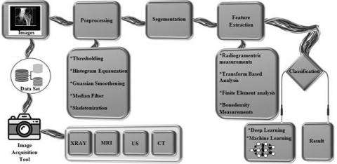
The classification of bone into osteoporosis, osteopenia, and normal bone using machine learning approaches is covered in this paper's assessment of DEXA image processing and other image processing techniques for osteoporosis detection. The general framework for the image processing technique is shown in Figure 1. DEXA images were used for image acquisition in order to construct the dataset. Dr. Sudhir Shah of Shah Orthopedic Hospital collected these images while maintaining patient privacy. This serves as a sample for illustrating bone mineral density (BMD). Preprocessing on this input image includes thresholding, histogram equalization, and filtering. Following segmentation, features are then retrieved using GLCM. AlexNet and DenseNet are two machine learning approaches that can be employed for classification.
Figure 1. General architecture of image processing
Numerous articles, books, and dissertations about osteoporosis detection have been published recently. This section discusses the relevant research.
2.1 DEXA image processing
One of the most widely used methods for detecting osteoporosis is DEXA, which can also be adopted to track how the body responds to treatment. It is helpful for determining body composition as well. DEXA screening can be used to measure BMD. Various methods for processing DEXA images have been developed in recent years. This section provides a concise overview of the fundamentals, modalities, procedures, and applications of DXA.
Two X-ray beams are produced by a DEXA system. One has a lot of energy, whereas the other has less. The DEXA scanner counts the total number of X-rays that come from both beams and pass through a bone. This is dependent on the bone's thickness. The difference between the two beams aids in determining the bone's T-Score, which in turn determines its bone mineral density. The T-range score's is as follows.
• T-score of -1.0 or above = normal bone density;
• T-score between -1.0 and -2.5 = low bone density, or osteopenia;
• T-score of -2.5 or lower = osteoporosis.
DXA and clinical challenges of fracture risk assessment in primary care [16].
Convolutional neural networks (CNNs), which employ the simulated DXA images to predict the histomorphometric properties of trabecular bone cubes, were first introduced by Xiao et al. [17]. The findings showed that CNN models were highly accurate in predicting histomorphometric parameters (from R = 0.80 to R = 0.985), indicating that DL models had the capacity to predict microstructural features from DXA images. This study also demonstrated that the number and resolution of the input simulated DXA images had a significant impact on the DL models' ability to predict results accurately. These results validated the study's hypothesis and proved that DXA images have a great deal of potential for predicting the likelihood of osteoporotic bone fracture. But the data used for the model was obtained from actual DEXA.
A 2D SSAM image processing method was created by Jazinizadeh et al. [18] to forecast hip fracture risk based on a single DXA scan. To take into account the influence of the femur's geometry and BMD distribution on the risk of hip fracture, 2D statistical shape and appearance modeling was carried out. In addition, the fracture risk was independently predicted using statistical shape modeling (SSM) and statistical appearance modeling (SAM) based only on the geometry and BMD distribution of the femur. The technique improved patient fragility diagnosis, as per the results. The number of parameters that could be analyzed to prevent non-convergence in the logistic regression was one of the techniques drawbacks, though. Parameters like T-score, BMD, Age, and Gender were adopted to estimate the FRAX score.
An artificial neural network for detection and prediction of osteoporosis was created by Tejaswini et al. [19]. The tibial bone underwent an impulse response test to look for osteoporosis. In participants with osteoporosis, the natural frequency of the vibration was much lower, which in turn suggested that the mechanical strength and mineral density of the bone had diminished. Therefore, this method is one of the crucial ones for detecting osteoporisis.
Tran et al. [20] introduced a regression artificial neural network (ANN) classifier-based computer-aided diagnosis (CAD) system for accurate osteoporotic risk detection on digital calcaneus radiographic images. The evaluation of this method's diagnostic ability involved identifying low BMD regions in the calcaneus region. 90% classification accuracy, sensitivity, specificity, and positive predictive value were all attained by this method. The calcaneus BMD may be predicted with high reliability and accuracy using this method.
2.2 Texture analysis for osteoporosis detection
Texture analysis is the process of identifying the ROI in an image based on its texture.
The third metacarpal bone and distal radius were automatically located and segmented using a region of interest (ROI) that Areeckal et al. [21] introduced to their automatic segmentation technique. Then, they employed cortical radiogrammetry, a low-cost pre-screening technology, to find people with low bone mass. Radiographs of the hand and wrist were taken to analyze the distal radius' trabecular texture and third metacarpal bone. The third metacarpal bone shaft was detected with an accuracy of 86% using the suggested automatic segmentation approach, and the distal radius ROI was located with an accuracy of 90%. Some images' segmentation failed because the radius and ulna bones in binary images were merged.
Harrar and Jennane [22] suggested a trabecular texture analysis using fractal metrics for bone fragility. Images from radiography tests were pre-processed using two different methods. To classify the two populations, the values of the fractal dimension and fractal signature were contrasted. The results showed that osteoporotic patients with a femoral fracture may be distinguished from controls using fractal analysis of texture on calcaneus radiographs. Comparing this discrimination to what was achieved by BMD alone, it was effective. But this approach did not take into account the characteristics of dynamic systems.
Kavitha et al. [23] combined the textural features and mandibular cortical width (MCW) derived from digital dental panoramic radiographs (DPRs), which performed better in screening for osteoporosis. 141 female patients' digital DPRs and bone mineral BMDs of the lumbar spine and femoral neck were used. In comparison to using simply individual data, the combination of textural features and MCW helped to improve the assessment of osteoporosis. In this investigation, only the lower border of the mandibular cortex, which is below the mental foramen, was utilized to compute the measurements of different textural aspects and MCW [24, 25].
2.3 Osteoporosis classification techniques
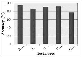
The technique of classifying a sample as impacted or unaffected, or as many results depending on the classifier design, is referred to as classification. The numerous classification methods were covered in Table 1. The various algorithms for each dataset and their constraints are briefly discussed. According to the table, ANN [25] obtained high accuracy (94%) than all other techniques, but EANN has a poor accuracy (85%).
Table 1. Various classification techniques
|
Author Name |
Key findings |
Datasets |
Results |
Drawbacks |
|
Aouache et al. [26] |
A fuzzy decision tree (FDT) model for Anterior osteoporosis (classes and severity) classification of the cervical radiography |
100 digitized cervical radiograph y images from NHANES II. |
Accuracy- 90.73% Lower accuracy- 0.4% |
The segmentation method based on the Active Shape Model was degrading the classification accuracy. |
|
Keerthika et al. [27] |
Artificial neural network (ANN) for Osteoporosis diagnosis |
Publicly available data. It contains the patient's history. |
Accuracy- 94% F1score- 96% Precision- 95% |
Predictive accuracy was low. |
|
Roberts et al. [28] |
Classification performance was assessed by ROC analysis. |
Existing dataset of 663 DPRs of female patients with (BMD) measurements. |
Accuracy- 85% sensitivity- 80% |
Low texture features were used for classification. |
|
Aliaga et al. [29] |
Fuzzy K- means classification. |
Patient’s X-ray images. |
Accuracy- 91% |
It was expensive for more iteration. |
|
Liu et al. [30] |
Ensemble Artificial Neural Networks (EANN) |
National Taiwan University Hospital with first low- trauma hip fractures patients. |
Accuracy – 85% Sensitivity- 88% |
Low prediction accuracy. |
|
Hatano et al. [31] |
Deep Convolutional Neural Network (DCNN) with CR images. |
101 cases of CR images. |
TPR: 64.7% and FPR: 6.51% |
High learning rate. |
Figure 2 illustrates the classification accuracy of DL techniques for osteoporosis detection on DEXA images. It can be seen that ANN [27] achieves an accuracy of 94%. In classification, EANN [30] and FDT [26] provide an accuracy of 85% and 90.73%, respectively.
Figure 2. Classification using deep learning techniques
3.1 Image acquisition
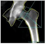
Image acquisition refers to the collection of the input databases. The DEXA scans of human skeletal remains are shown here. 600 or so samples are provided by an orthopedic surgeon for DEXA imaging. Random noises are applied to the gathered images. For medical imaging systems, the most challenging task is imperfect acquisition and transmission problems brought on by the tampering of visual signals. To enhance the quality of the image, these distortions—which are referred to as "Noise"—must be eliminated. "Image denoising" refers to the noise-reduction methods. Medical imaging has not been explored as much as image denoising, an issue in computer vision for natural images that has received considerable attention. As noisy images frequently result in wrong diagnosis, it is the tool that image analyzers in the quickly expanding medical profession most frequently seek for. Figure 3 shows the input image of this research.
Figure 3. Input image
3.2 Image preprocessing
The RGB images of the collected X-rays are changed into grayscale images. Gaussian noise, salt and pepper noise, and other types of noise are exhibited in the images prior to conversion. Among these, salt and pepper noise is the most prevailing noise of the X-ray images.
3.2.1 RGB to the gray-scale conversion
The image is imported into matrix form as w * h * c, where w stands for image width, h for image height, and c for channel count. While color images have three channels, including red, green, and blue colors, grayscale images only have one channel, which is black and white. The image matrix needs to be guaranteed to remain constant and persistent throughout the application. The image matrix uses these global variables to reduce the rate of collinearity.
3.2.2 Median filtering
It is one of the effective methods for making the salt and pepper noises work. The technique functions similarly to a nonlinear digital filtering approach that removes noise. After noise removal, median filtering is applied to these images. It helps to preserve the edges of the images, even after applying impulsive noise to them. The size and form of the filtering mask have an impact on the median filter's ability to reduce noise. This filter has a rank order component as well. An image is examined pixel by pixel, and each value is replaced with the median value of the adjacent pixels [32]. The pattern of neighbors is referred to as a "window." The window moves over the full image pixel by pixel. The median value is determined by first placing all of the window's pixel values in numerical order, and then substituting the middle (median) pixel value for the one being considered. The output of average and median filtering is illustrated in Figure 4.
Figure 4. Output of average and median filtering
3.3 Image segmentation
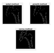
The filtered input X-ray image then goes through segmentation by three models, namely, Sobel edge detection, Prewitt edge detection, and Canny edge detection.
3.3.1 Sobel edge detection
To determine the gradient of the images, a Sobel edge detection technique is used. It is a novel gradient computation of a certain kind that fixes the problems with image edge detection. In our investigation, the template convolution process is performed on a 3*3-pixel area. The gradient values of the central pixel are then contrasted with the gradient values of the predefined threshold. There are two sets in the convolution template, one at the level edge of detection and the other for the vertical edge of detection [21, 33-35].
Since it operates on the gradient expression and the f(x,y) two-dimensional image function, it is presented as follows:
The gradient integration can be expressed as:
The gradient of the pixel is the estimated synthetic gradient G. There are two models that it uses to represent the gradient values. The pseudocode of Sobel edge detection is as follows:
Step 1: Get the input image.
Step 2: Applying Gx and Gy masks to the input image.
Step 3: Use the gradient of the Sobel edge detection technique.
Step 4: Separately manipulate the Gx and Gy masks on the provided image.
Step 5: Merge the results to calculate the gradient's absolute magnitude.
Step 6: The output edges now represent absolute magnitude.
3.3.2 Prewitt edge detection
The Prewitt operator is utilized to determine the gradient of the picture intensity function. Never does it place pixels that are closer to the mask's center. Its two parts, namely, vertical edge component and the horizontal edge component, are calculated using kernels Gx and Gy, respectively. The gradient's intensity in the current pixel is indicated by |Gx| + |Gy|. There are only 8 permitted directions. Prewitt is a gradient-centered edge detector that makes estimates for eight directions in the 3×3 neighborhood. Complete eight convolution masks are produced, and one complication mask is chosen from these eight masks with the persistence of the module, which is principal. In comparison to Sobel detection, this edge detection technique is straightforward. The only defect is the creation of more noises.
3.3.3 Canny edge detection
It is the most effective and efficient edge detection method. It smoothens an image with a Gaussian filter. Next, the Prewitt and Sobel edge operators' outputs are used to approximate the magnitude and angle of gradients. The non-maxima suppression is used to measure the gradient magnitude. To identify the strong and weak edge pixels, two thresholding operations are used. The weak borders of the pixels are removed [36-38]. Edges are discovered with Canny by removing noise from an image. This does not change the features of the image edges.
The algorithmic steps are as follows [30]:
• Convolve image f(r, c) with a Gaussian function to get smooth image f^(r, c).
f^(r, c)=f(r,c)*G(r,c,6)
• Apply first difference gradient operator to compute edge strength then edge magnitude
and direction are obtained as before.
• Apply non-maximal or critical suppression to the gradient magnitude.
• Apply threshold to the non-maximal suppression image.
Canny edge detector is not very susceptible to noise.
3.3.4 K-means segmentation
After determining which object segmentation method works best, a k-mean clustering strategy is used to get the best segmented image possible. The steps are:
(1) Calculate the number of clusters, which determines the k-value.
(2) Distribute the image pixels across the k-clusters at random.
(3) Estimate the cluster's center image data points;
(4) Estimate the distance between the image data points towards the cluster center;
(5) The image data points are reorganized before locating the clusters based on the estimated distance from the clusters.
(6) The cluster centers are positioned similarly [31, 37].
Figures 5-8 show the output of the segmentation method, the gradient method, the Laplacian method, and the k-means segmentation, respectively.
Figure 5. Output of the segmentation method
Figure 6. Output of the gradient method
Figure 7. Output of the Laplacian method
Figure 8. Output of the k-mean segmentation
3.4 Features extraction
Important features are extracted from the segmented image. Here, the intrinsic and extrinsic statistical data of a segmented image are discovered using a gray level co-occurrence matrix (GLCM). It is a second-order measure that investigates an image's textural features. The textures' grey levels are sampled to extract the features of the image. The co-occurrence matrix displays the extracted features. The estimated texture features are then calculated using the matrix created in the preceding step. The formulas for calculating these attributes are provided in Table 2. Figure 9 shows the shape-based textural features measured using GLCM.
Table 2. Feature extraction formulas for the segmented image
|
Extracted features |
Formulae |
|
Contrast |
$\sum_{i, j=0}^{N-1} P_{i j}(i-j)^2$ |
|
Correlation |
$\sum_{i, j=0}^{N-1} P_{i j}\left[\frac{\left(i-\mu_j\right)\left(j-\mu_j\right)}{\sqrt{\left(\sigma_i^2\right)\left(\sigma_j^2\right)}}\right.$ |
|
Energy |
$\sum_{i=0}^{N-1}[P(i)]^2$ |
|
Homogenity |
$\sum_{i, j=0}^{N-1} \frac{P_{i j}}{1+(i-j)^2}$ |
|
Mean |
$\sum_{i=0}^{N-1} z_i p\left(z_i\right)$ |
|
Standard Deviation ($\sigma^2$) |
$\sum_{i=0}^{N-1}\left(z_i-m\right)^2 p\left(z_i\right)$ |
|
Entropy |
$\sum_{i=0}^{N-1}-\ln \left(P_{i j}\right) P_{i j}$ |
|
Kurtosis |
$\sum_{i=0}^{N-1}\left(z_i-m\right)^4 p\left(z_i\right)$ |
|
Skewness |
$\sum_{i=0}^{N-1}\left(z_i-m\right)^2 p\left(z_i\right)$ |
|
IDM |
$\sum_{i, j} \frac{P_{i, j}}{1+(i-j)^2}$ |
Figure 9. Shape-based textural features measured using GLCM
3.5 Deep learning classification
Here, radiological features of human bones are predicted using CNNs with the AlexNet classifier model and DenseNet. Image features are imported to CNN as essential inputs. The CNN consists of an input layer, an output layer, and a number of hidden levels, totaling three layers. Each layer operates according to its own set of features for learning. Convolution, activation or ReLU, and pooling are the three most prevalent layers in CNN.
a) Convolution is a set of convolutional filters for activating certain features.
b) ReLU maps the negative values to zero and administers the positive values. These values are further processed onto activation layers.
c) The pooling layer identifies the variant features through nonlinear down-sampling [31].
Here, AlexNet and DenseNet are the two designs that are utilized. Eight layers make up the AlexNet architecture, five of which are convolutional and three of which are fully connected. The 11-by-11 filter size is employed in the first convolutional layer for convolution and max-pooling. With 3-by-3 filters and a stride size of 2, the max-pooling procedures are carried out. The same procedures are also performed out by the second layer, which has a 5-by-5 filter layer. The 3-by-3 filters employed in the max-pooling processes have a stride size of 2. In the third, fourth, and fifth convolutional layers, the filter size is 3-by-3. At the fifth layer, 3-by-3 filters with a stride size of 2 are used for the max-pooling operations. 4,096 neurons constitute each of the sixth and seventh fully connected layers. The first seven layers each have the ReLU activation function implemented. The sixth and seventh layers are given a dropout ratio of 0.5. Finally, a softmax function receives the eighth layer output [36]. Dropout is a regularization method to get around the overfitting issue that persists in deep neural networks. As a result, each epoch's training duration is cut down.
DenseNet consists of 3 essential building blocks: input and output layers for enabling scalability, transition layers for supporting scalability, and dense blocks, which are the key elements of the method. The previously discussed connection pattern is achieved using dense blocks, where each layer is connected to each layer below it in a feedforward manner.
This section presents the experimental setup and performance measures of the study. The proposed technique is implemented in MATLAB, a high-level simulation language. The results of AlexNet are displayed in Figure 10.
The results of DenseNet are displayed in Figure 11.
Figure 10. Results of AlexNet
Figure 11. Results of DenseNet
A common technique for detecting osteoporosis is DEXA, which measures BMD using a simpler, quicker, and non-invasive approach. The following table compares the results of the classification methods AlexNet and DenseNet. The studied algorithm used datasets of the size 600 ffor the prediction. Both training and testing were carried out on the input dataset. The detection performance was verified through comparative analysis. Classification accuracy, sensitivity, and F-measure were selected to examine the performance of AlexNet and DenseNet. Table 3 and Figure 12 show the performance measures and achieved results.
Table 3. Performance measures and achieved results
|
Performance metrics |
AlexNet |
DenseNet |
|
ROC |
96.9664 |
93.5903 |
|
Accuracy |
94.7368 |
95.1754 |
|
Error |
10.5263 |
9.6491 |
|
Sensitivity |
89.0508 |
89.2297 |
|
Specificity |
96.3127 |
96.5123 |
|
Precision |
89.8754 |
91.8971 |
|
False positive rate |
3.6873 |
3.4877 |
|
F-score |
89.4023 |
90.2416 |
Figure 12. Graphical representation of performance measures and achieved results
Osteoporosis is one of the deadliest diseases in the world. The diagnosis of osteoporosis is challenging in the majority of nations due to issues like the lack of a reference database, the cost of the scanning equipment, the lack of skilled technical personnel, etc. Preprocessing, feature extraction, and classification are the steps that are used in vision-based diagnosis, and they are all covered in this article. Although DEXA is one of the most widely used methods for detecting osteoporosis, it has certain drawbacks, such as difficulty in interpreting scan data. It cannot forecast the danger of fracture (Youngs Modulus). With the use of image processing of human bone, this paper proposes a method for the comparative investigation of mechanical and radiological features. This disease can be managed in the future by raising awareness, preventing the condition with a healthy diet and treatment, improving categorization accuracy, and having a wide range of affordable, effective equipment available.
[1] Ali, G.Y., Abdelbary, E.E., Albuali, W.H., AboelFetoh, N.M., AlGohary, E.H. (2017). Bone mineral density & bone mineral content in Saudi children, risk factors and early detection of their affection using dual-emission X-ray absorptiometry (DEXA) scan. Egyptian Pediatric Association Gazette, 65(3): 65-71. https://doi.org/10.1016/j.epag.2017.03.005
[2] Carey, J.J., Delaney, M.F. (2017). Utility of DXA for monitoring, technical aspects of DXA BMD measurement and precision testing. Bone, 104: 44-53. https://doi.org/10.1016/j.bone.2017.05.021
[3] Cox, S.I., Hooper, G. (2020). Improving bone health and detection of osteoporosis. The Journal for Nurse Practitioners, 17(2): 233-235. https://doi.org/10.1016/j.nurpra.2020.05.008
[4] Czyz, M., Kapinas, A., Holton, J., Pyzik, R., Boszczyk, B.M., Quraishi, N.A. (2017). The computed tomography-based fractal analysis of trabecular bone structure may help in detecting decreased quality of bone before urgent spinal procedures. The Spine Journal, 17(8): 1156-1162. https://doi.org/10.1016/j.spinee.2017.04.014
[5] Hoff, B.A., Kozloff, K.M., Boes, J.L., Brisset, J., Galbán, S., Van Poznak, C.H., Jacobson, J.A., Johnson, T.D., Meyer, C.R., Rehemtulla, A., Ross, B.D., Galbán, C.J. (2021). Parametric response mapping of CT images provides early detection of local bone loss in a rat model of osteoporosis. Bone, 51(1): 78-84. https://doi.org/10.1016/j.bone.2012.04.005
[6] Edmondson, C.P., Schwartz, E.N. (2017). Non-BMD DXA measurements of the hip. Bone, 104: 73-83. https://doi.org/10.1016/j.bone.2017.03.050
[7] Li, L., Wong, K., Law, M.W., Fang, B.X., Lau, V.W., Vardhanabuti, V.V., Lee, V.K., Cheng, A.K., Ho, W., Lam, W.W. (2018). Opportunistic screening for osteoporosis in abdominal computed tomography for Chinese population. Archives of Osteoporosis, 13(1): 1-7. https://doi.org/10.1007/s11657-018-0492-y
[8] Lee, D.C., Hoffmann, P.F., Kopperdahl, D.L., Keaveny, T.M. (2017). Phantomless calibration of CT scans for measurement of BMD and bone strength—inter-operator reanalysis precision. Bone, 103: 325-333. https://doi.org/10.1016/j.bone.2017.07.029
[9] Rud, B., Vestergaard, A., Hyldstrup, L. (2016). Accuracy of densitometric vertebral fracture assessment when performed by DXA technicians—a cross-sectional, multiobserver study. Osteoporosis International, 27(4): 1451-1458. https://doi.org/10.1007/s00198-015-3395-4
[10] Sela, E.I., Pulungan, R. (2019). Osteoporosis identification based on the validated trabecular area on digital dental radiographic images. Procedia Computer Science, 157: 282-289. https://doi.org/10.1016/j.procs.2019.08.168
[11] Tecle, N., Teitel, J., Morris, M.R., Sani, N., Mitten, D., Hammert, W.C. (2020). Convolutional neural network for second metacarpal radiographic osteoporosis screening. The Journal of Hand Surgery, 45(3): 175-181. https://doi.org/10.1016/j.jhsa.2019.11.019
[12] Zhang, N., Magland, J.F., Rajapakse, C.S., Lam, S.B., Wehrli, F.W. (2013). Assessment of trabecular bone yield and post-yield behavior from high-resolution MRI- based nonlinear finite element analysis at the distal radius of premenopausal and postmenopausal women susceptible to osteoporosis. Academic Radiology, 20(12): 1584-1591. https://doi.org/10.1016/j.acra.2013.09.005
[13] Mrgan, M., Mohammed, A., Gram, J. (2013). Combined vertebral assessment and bone densitometry increases the prevalence and severity of osteoporosis in patients referred to DXA scanning. Journal of Clinical Densitometry, 16(4): 549-553. https://doi.org/10.1016/j.jocd.2013.05.002
[14] Schousboe, J.T., Riekkinen, O., Karjalainen, J. (2017). Prediction of hip osteoporosis by DXA using a novel pulse-echo ultrasound device. Osteoporosis International, 28(1): 85-93. https://doi.org/10.1007/s00198-016-3722-4
[15] Liu, J., An, F. (2020). Image classification algorithm based on deep learning-kernel function. Scientific Programming, 2020: 7607612. https://doi.org/10.1155/2020/7607612
[16] Williams, S., Khan, L., Licata, A.A. (2021). DXA and clinical challenges of fracture risk assessment in primary care. Cleveland Clinic Journal of Medicine, 88(11): 615-622. https://doi.org/10.3949/ccjm.88a.20199
[17] Xiao, P., Zhang, T., Dong, X.N., Han, Y., Huang, Y., Wang, X. (2020). Prediction of trabecular bone architectural features by deep learning models using simulated DXA images. Bone Reports, 13: 100295. https://doi.org/10.1016/j.bonr.2020.100295
[18] Jazinizadeh, F., Adachi, J.D., Quenneville, C.E. (2020). Advanced 2D image processing technique to predict hip fracture risk in an older population based on single DXA scans. Osteoporosis International, 31(10): 1925-1933. https://doi.org/10.1007/s00198-020-05444-7
[19] Tejaswini, E., Vaishnavi, P., Sunitha, R. (2016). Detection and prediction of osteoporosis using impulse response technique and artificial neural network. In International Conference on Advances in Computing, Communications and Informatics (ICACCI), IEEE, pp. 1571-1575. https://doi.org/10.1109/ICACCI.2016.7732272
[20] Tran, D., Rutledge, D.N., Robertson, S. (2019). Prediction of osteoporosis among Vietnamese women. The Journal for Nurse Practitioners, 15(5): 361-364. https://doi.org/10.1016/j.nurpra.2019.01.017
[21] Vishnu, T., Saranya, K., Arunkumar, R., Gayathri Devi, M. (2015). Efficient and early detection of osteoporosis using trabecular region. 2015 Online International Conference on Green Engineering and Technologies (IC-GET). http://doi.org/10.1109/GET.2015.7453840
[22] Areeckal, A.S., Kamath, J., Zawadynski, S., Kocher, M. (2018). Combined radiogrammetry and texture analysis for early diagnosis of osteoporosis using Indian and Swiss data. Computerized Medical Imaging and Graphics, 68: 25-39. https://doi.org/10.1016/j.compmedimag.2018.05.003
[23] Harrar, K., Jennane, R. (2015). Quantification of trabecular bone porosity on X-ray images. Journal of Industrial and Intelligent Information, 3(4): 280-285. https://doi.org/10.12720/jiii.3.4.280-285
[24] Kavitha, M.S., An, S.Y., An, C.H., Huh, K.H., Yi, W.J., Heo, M.S., Lee, S.S., Choi, S.C. (2015). Texture analysis of mandibular cortical bone on digital dental panoramic radiographs for the diagnosis of osteoporosis in Korean women. Oral surgery, Oral Medicine, Oral Pathology and Oral Radiology, 119(3): 346-356. https://doi.org/10.1016/j.oooo.2014.11.009
[25] Wani, I.M., Arora, S. (2020). Computer-aided diagnosis systems for osteoporosis detection: A comprehensive survey. Medical & Biological Engineering & Computing, 58(9): 1873-1917. http://doi.org/10.1007/s11517-020-02171-3
[26] Aouache, M., Hussain, A., Zulkifley, M.A., Zaki, D.W.M.W., Husain, H., Hamid, H.B.A. (2018). Anterior osteoporosis classification in cervical vertebrae using fuzzy decision tree. Multimedia Tools and Applications, 77(3): 4011-4045. https://doi.org/10.1007/s11042-017-4468-5
[27] Keerthika, P., Suresh, P., Manjula Devi, R., Gunavathi, C., Senapathi, T., Praveen Kumar, R., Nikhil, V. (2020). An intelligent bio-inspired system for detection and prediction of osteoporosis. Materials Today: Proceedings, 45: 2010-2016. https://doi.org/10.1016/j.matpr.2020.09.477
[28] Roberts, M.G., Graham, J., Devlin, H. (2013). Image texture in dental panoramic radiographs as a potential biomarker of osteoporosis. IEEE Transactions on Biomedical Engineering, 60(9): 2384-2392. https://doi.org/10.1109/TBME.2013.2256908
[29] Aliaga, I., Vera, V., Vera, M., García, E., Pedrera, M., Pajares, G. (2020). Automatic computation of mandibular indices in dental panoramic radiographs for early osteoporosis detection. Artificial Intelligence in Medicine, 103: 101816. https://doi.org/10.1016/j.artmed.2020.101816
[30] Liu, Q., Cui, X., Chou, Y., Abbod, M.F., Lin, J., Shieh, J. (2015). Ensemble artificial neural networks applied to predict the key risk factors of hip bone fracture for elders. Biomedical Signal Processing and Control, 21: 146-156. https://doi.org/10.1016/j.bspc.2015.06.002
[31] Hatano, K., Murakami, S., Lu, H., Tan, J.K., Kim, H., Aoki, T. (2017). Classification of osteoporosis from phalanges CR images based on DCNN. In 17th International Conference on Control, Automation and Systems (ICCAS), IEEE, pp. 1593-1596. https://doi.org/10.23919/ICCAS.2017.8204241
[32] Muthukrishnan, R., Radha, M. (2011). Edge detection techniques for image segmentation. International Journal of Computer Science & Information Technology (IJCSIT), 3(6): 259-267. https://doi.org/10.5121/ijcsit.2011.3620
[33] Mendiratta, S., Turk, N., Bansal, D. (2023). Robust feature extraction and recognition model for automatic speech recognition system on news report dataset. In: Joshi, A., Mahmud, M., Ragel, R.G. (eds) Information and Communication Technology for Competitive Strategies (ICTCS 2021). Lecture Notes in Networks and Systems, vol 400. Springer, Singapore. https://doi.org/10.1007/978-981-19-0095-2_56
[34] Dixit, A., Kasbe, T. (2022). Multi-feature based automatic facial expression recognition using deep convolutional neural network. Indonesian Journal of Electrical Engineering and Computer Science, 25(3): 1406-1419. http://doi.org/10.11591/ijeecs.v25.i3.pp1406-1419
[35] Zhang, K., Zhang, Y., Wang, P., Tian, Y., Yang, J. (2018). An Improved Sobel Edge Algorithm and FPGA Implementation. Procedia Computer Science, 131: 243-248. https://doi.org/10.1016/j.procs.2018.04.209
[36] Guo, C., Xu, Y., Tian, Z. (2020). Inversion of PM2.5 atmospheric refractivity profile based on AlexNet model from the perspective of electromagnetic wave propagation. Environmental Science and Pollution Research, 27: 37333-37346. https://doi.org/10.1007/s11356-020-07703-w
[37] Sumathi, A., Kowsalya, K., Srinithi, K.P., Sudarvizhi, M. (2019). Performance analysis of clustering algorithms for MRI brain images. 2019 International Conference on Intelligent Sustainable Systems (ICISS). https://doi.org/10.1109/ISS1.2019.8907943
[38] Xiao, P., Zhang, T., Dong, X.N., Han, Y., Huang, Y., Wang, X. (2020). Prediction of trabecular bone architectural features by deep learning models using simulated DXA images. Bone Reports, 13: 100295. https://doi.org/10.1016/j.bonr.2020.100295