Yong Zhang
© 2022 IIETA. This article is published by IIETA and is licensed under the CC BY 4.0 license (http://creativecommons.org/licenses/by/4.0/).
OPEN ACCESS
A fully automatic plug seedling device is designed, its structure and working principle are introduced, and a plug seedling hole identification method based on CNN is proposed to address the issue of adjacent holes in order to increase the automation and intelligence of the vegetable transplanting machine. The issue of low recognition accuracy of plug seedlings is brought on by intertwined stems and leaves. This study first grows tomato seedlings in an artificial greenhouse and then utilizes an SLR camera to take pictures of those plants. The photos are then subjected to the appropriate preprocessing, such as separating the complete hole plate image into several hole images in accordance with the hole plate standards to facilitate recognition. The CNN model is then finished being trained after receiving the processed image. Relu, which has a better ability for classification, is chosen as the activation function of the convolutional layer after the network is enlarged on the basis of LeNet-5CNN. In addition, the over-fitting issue of the model is resolved using data augmentation technology, resulting in a recognition accuracy of the test set of the model that is as high as 0.985. The automatic vegetable transplanting machine can greatly increase the automation and intelligence level of the plug seedling recognition model based on CNN, which has high recognition accuracy and generalization ability. This model also solves the main technical problems of the plug seedling device and improves the machine's ability to transplant.
plug seedling device, plug seedling identification, convolutional neural network, regularization, data enhancement
The world's largest producer of vegetables is China. The primary planting technique used in vegetable production is plug seedling transplantation. More and more mechanized transplanting is employed as planting volume and labor costs rise. The majority of transplanting devices are semi-automatic devices that require manual seedling feeding and cannot effectively address the issues of high labor intensity, poor transplanting efficiency, or poor transplanting precision. Vegetable seedlings are automatically removed from the hole tray by the automatic transplanting machine, which then plants them in larger pots or fields. Due to its benefits of having a high transplanting efficiency and low labor intensity, it has drawn the attention of relevant institutions for research. However, there will be holes, weak seedlings, and residual seedlings in the plug tray due to factors including seed germination rate and seedling habitat. It will still be transplanted normally if the automatic transplanting device is unable to detect the holes. It will significantly reduce the automatic transplanting machine's ability to transplant, increasing the likelihood of missed planting. It is therefore possible to increase the automation and intelligence level of the automatic transplanting machine, which is the key to improving automatic transplanting, by identifying and judging whether each hole in the hole plate is suitable for transplanting and filling pot seedlings of the same age into the holes that are not suitable for transplanting, creating a successful method for machine transplantation.
Research on plug seedling identification has been done by academics and organizations associated to it both domestically and overseas. An automatic transplanting device supported by machine vision was created by Tai et al. [1]. The segmentation threshold was established by sampling based on the image's gray information to assess whether the hole is empty. A seedbed transplanting robot with a vision system was created by Ryu et al. [2] and employs a predefined value for image segmentation to locate holes to speed up transplanting. The Futura fully automatic transplanting device from Ferrari, Italy, scans the plug seedling using photoelectric technology to assess whether there are enough seedlings. A detecting system using a background suppression diffuse reflection photoelectric sensor was created by Wu et al. and Jin [3, 4]. In order to determine whether there are enough seedlings, the sensor can alter the height and detecting distance at which it looks for the stems of the first row of plug seedlings. A plug seedling form parameter measurement system based on line structured light vision was created by Feng et al. [5]. The plug seedling image was processed using 2G-R-B, and the leaf and background were determined after a dynamic threshold for segmentation of the leaf and background was obtained using the maximum between-class variance approach. A machine vision system was created by Jiang et al. [6] to monitor the growth of plug seedlings in the pot-moving robot. A watershed method based on morphology was created to segment the edge of the leaf while avoiding the influence of nearby holes. To determine whether a seedling is ready for transplantation, it is necessary to measure its girth and leaf area. In order to determine if there were seedlings in the holes, Wang et al. [7] grayscaled the Arabidopsis plug seedling image, obtained a binary image using the Otsu threshold segmentation method, and then counted the image pixels of the seedlings in the holes. Two categories of detection methods are used in the research mentioned above. One is the use of photoelectric sensors, although this technology can only identify the absence of seedling data. a smaller extent. The second approach uses image processing. The aforementioned image processing techniques base their calculation of the quantity of leaf pixels in the hole on picture segmentation [8]. However, following image segmentation the seedlings will be lost due to the effects of light, shooting angle, and plug seedling matrix. It is better to identify early plug seedlings because some stems, leaves, and the coherence information between stems and leaves are easily influenced by adjacent holes.
In the middle and early stages of vegetable plug seedling cultivation, the plug seedlings are typically replanted. The plug seedlings will overlap in the center or middle early stage because they grow more quickly. Therefore, a more accurate method of plug seedling identification is needed. As one of the most efficient learning techniques in the field of machine learning, CNN [9] (convolutional neural network) has gained popularity in recent years. Its learned features have translation invariant qualities and can learn objects. It performs better in the field of picture recognition because of the spatial hierarchy. Research into CNN's use in agriculture has also been conducted by an increasing number of academics. Wang et al. [10] employed CNN to the identification of corn weeds, Ma et al. [11] used CNN to identify greenhouse cucumber illnesses, CNN was used to classify and identify banana leaf diseases by Amara et al. [12] and Brahimi et al. [13] for the identification of tomato illnesses.
This paper first introduces the structure and operating principle of the plug seedling device based on machine vision, then goes into detail about the image acquisition and data set preprocessing process, and finally inputs the preprocessed plug seedling image into CNN, using the model's powerful feature extraction ability, to solve the problem of mutual interference of adjacent hole seedlings, determine whether the hole is a hole, and provide a guide for impromptu experiments.
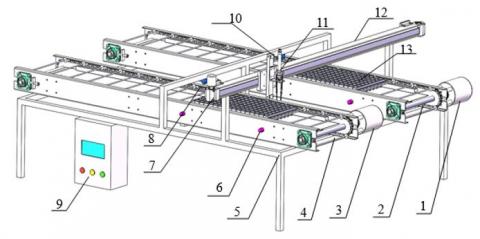
Figure 1 depicts the structure of the plug seedling device. A control box, a vision system, a conveyor belt, and a photoelectric switch for a manipulator are the essential components. The device's overall control is realized via the control box. The vision system for plug seedlings is made up of an industrial camera and an industrial computer. The manipulator is fixed to the linear module, the linear module is driven by the servo motor to realize actions such as grasping and replenishing the seedlings, and the seedling tray is realized by the photoelectric switch. The identification and the transport of the seedling tray are completed by the conveyor belt and stepping motor, respectively.
The No. 1 transmission belt seedling tray's potted seedlings appropriate for transplant are removed by the seedling device and placed on the No. 2 transmission belt seedling tray. When filling seedling trays, the operator inserts the trays on conveyor belts No. 1 and No. 2, and the two conveyor belts operate independently to move the trays to the right beneath the camera. After correctly identifying and judging a plug seedling, the visual system notifies the controller with a recognition message. data, after which the seedling tray is transported to the manipulator's base by the conveyor belt. Under the controller's control, the manipulator moves to the No. 2 conveyor belt seedling tray first, removing the substrate from the holes that are unsuitable for transplanting. The manipulator then moves to the middle of the two conveyor belts, discarding the substrate, before moving to the No. 1 conveyor belt. Take the pot seedlings that are ready for transplanting off the seedling tray, then quickly run to the No. 2 conveyor belt and place the pot seedlings there. To carry out the seedling replenishment operation, the seedling device's conveyor belt, linear module, and manipulator cooperate and move back and forth under the controller's control. The controller issues an audible and visual alarm to remind the operator to remove or supply fresh seedling trays in time when the seedling tray on the second conveyor belt is full or when there is no pot seedling appropriate for transplanting on the seedling tray on the No. 1 conveyor belt.
Figure 1. Structure diagram of seedling supplement device
3.1 Image acquisition
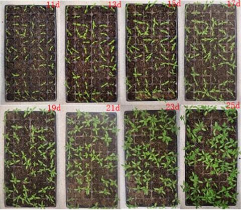
Tomato seedling photos were trained on in this study. Tomato seedlings were grown in four trays in a makeshift greenhouse. The greenhouse was maintained at a constant 25°C during the day and 15°C at night. The tray has a 12 by 6-hole design. A Canon 550D single-lens reflex camera with 18 million pixels is used for the image collection. A rack with a 50 cm height is used to position the camera exactly over the seedling tray. On October 8, 2018, seeds were seeded, and on October 19, image collection got underway. By altering the artificial greenhouse's light intensity during the image collection process, the light changes that occurred while the plug seedling device was operating indoors were replicated. During the 10- to 28-day seedling cultivation phase, a total of 581 photos of tomato seedlings were captured from various angles. Figure 2 shows a picture of tomato seedlings at their 11–25 day seedling stage. For only three days, the tomato seedlings in the 11-day seedling stage had been uncovered. The image shows that at this point, the length of the tomato seedlings' two leaves is roughly equal to the width of the hole, and while some seedlings have spread to neighboring holes, they are essentially distributed inside their own hole region. In the 25-day image of the seedling raising period, the overlapping of adjacent holes is serious, but the outline of the holes is basically clear, and whether the holes are empty can still be judged through the information of the stems and leaves of the seedlings.
Figure 2. Tomato seedling image
3.2 Image preprocessing and dataset construction
The original image of the gathered tomato seedlings is 3264 x 1840 pixels in size. The scale of the CNN model will be very large if the original image is directly recognized because it is relatively large; if the resolution is decreased, a lot of feature information will be lost and the recognition accuracy will decrease. Since the goal of the model recognition in this paper is to determine whether the hole is empty, the method of dividing the large hole plate image into small single hole images is adopted in order to decrease the difficulty of recognition and improve recognition accuracy, so that the network model only needs to identify the hole. The plug seedling recognition is converted into a binary classification problem whether the hole picture is empty or not, and the small image still has a high resolution, saving the majority of the stem and leaf information of the seedlings, which may assure the accuracy of the recognition.
Figure 3 depicts the creation of the data collection and the picture preparation procedure. The non-seedling plate portion of the original image is first removed, and then, in accordance with the requirements of the seedling plate, it is divided into 72 separate images, each measuring 12 by 6, along the edge of the hole. The split image is a file in the JPEG format, and the image corresponds to a hole. The size is 128128 pixels, the depth is 3, and the value is in a tensor of floating point values between 0 and 1, after the RGB format conversion, size correction, conversion of floating point numbers, and 01 normalization procedure. The plug seedling device performs the aforementioned picture preprocessing operation. The industrial computer's automatic processing can be achieved by position calibration since the hole plate stops directly under the camera, fixing its position.
Each tomato seedling image has a hole-to-no-hole ratio of roughly 1:5. The number of holes and non-hole photos in the training set and test set are equal, and 4000 images from the preprocessed images of tomato seedlings were chosen as the training set and 1000 images were used as the test set in order to confirm that this study is a balanced binary classification.
Figure 3. Image preprocessing flow and data set construction process
When a plug seedling is discovered, segmentation techniques like color can be used to realize hole identification since, if the plug seedling is small, its stems and leaves are primarily distributed in its own hole area. The red arrow in Figure 3 illustrates how the plug seedling expands outward after reaching a particular stage of growth, at which point the stems and leaves of nearby holes will overlap. The research reveals that the split hole image comprises the seedlings' stems in addition to their leaves, and that the holes may be located by identifying the traits of the stems and leaves. However, because the stalk is so thin and nearly the same color as the substrate, it is challenging to extract characteristics using color segmentation and other methods. In order to achieve hole recognition through its potent feature extraction capability, a CNN recognition model is constructed in this study.
4.1 Principle of CNN
The input layer, convolutional layer, pooling layer, fully connected layer, and output layer make up the majority of a CNN. A collection of training images are entered into the input layer. The essential component of CNN is the convolutional layer, which typically consists of numerous 33 or 55 convolution kernels. You can think of the convolution kernel as a feature extractor. Only local features of the image may be extracted by the convolution kernel because of its limited size. The convolutional layer may, however, extract numerous local features from the image by increasing the number of convolution kernels. After feature extraction, the convolutional layer can then be used for identification anywhere else in the image. The convolutional layer closest to the input layer learns the smaller local features, while the subsequent convolutional layer learns the bigger image features based on the features of the previous convolutional layer. CNN typically consists of numerous convolutional layers. The pooling layer's primary job is to downscale the number of model parameters while maintaining the model recognition impact. The output layer contains a classifier that outputs the model's final recognition result, and the fully connected layer extracts the overall image features from the convolutional layer [14].
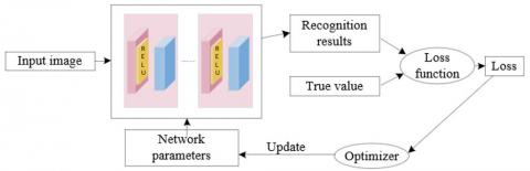
In order to accomplish certain tasks through training, CNN needs the right network parameters after determining the network design. Loss function and an optimizer are used to implement network parameter training. Figure 4 depicts the connection between the network design, loss function, and optimizer. The loss function determines the loss value by calculating the difference between the network recognition result and the real value. The network parameters are updated by the optimizer using the loss value and training data. The loss function is also referred to as the objective function because the optimizer's ultimate objective is to minimize the loss value.
4.2 Construction of identity model
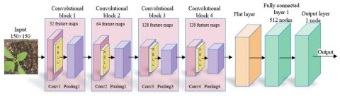
One of the oldest models, the CNN model LeNet-5 [15], was initially employed for handwritten digit recognition. This study expands the LeNet-5 network and creates a CNNplug seedling recognition model. Figure 5 depicts the model structure, while Table 1 displays the model parameters. The model consists of four convolutional blocks, with a convolutional layer, an activation layer, and a pooling layer in each block. The stride of the convolution operation is set to 1, and the convolution layer employs a 33 convolution kernel. A feature map is created from the input data after convolution. There are 32, 64, 128 and 128 feature maps, respectively. The graph keeps growing, but as the convolution operation continues, its size steadily shrinks. With maximum pooling downsampling, a 22 window, and a stride of 2, the pooling layer shrinks the feature map to half its original size. The convolutional block's multidimensional tensor is converted into a one-dimensional tensor via the flattening layer. The 512 neuron-node fully connected layer incorporates the feature maps found by the convolutional layer. An activation function layer is also included in this layer. The final classification outcome is produced from the output layer, which is also a fully connected layer and contains just one neuron node.
4.3 Recognition model optimization
CNN requires optimization, loss, activation, and other functions. There are numerous different types of each function. The right function must be chosen based on the application in order to get the best performance out of the model.
4.3.1 Activation function
The model can do nonlinear modeling thanks to the activation function. In this study, sigmoid functions, exponential linear units, and rectified linear units (Relu, Relu, and Elu, respectively) are used [16, 17].
Relu is one of the activation functions that is now employed the most, and the expression is shown in formula (1). Since only some neurons are active when the input is negative, the network's capacity is decreased and computational efficiency is increased. This is evident from the statement that when the input is a negative number, its output is 0, and the corresponding neurons will not be activated.
$R\left(x_i\right)= \begin{cases}0 & \left(x_i \leq 0\right) \\ x_i & \left(x_i>0\right)\end{cases}$ (1)
Formula (2) illustrates the activation function Elu's expression. This function is an improvement over the Relu function. It is effective for input changes and noise because Elu and Relu are equal in the interval of x>0 and its output is not zero in the interval of x0. It has a higher level of resilience, and because the mean value of its output is closer to 0, it converges more quickly.
${Elu}\left(x_i\right)= \begin{cases}\alpha\left(\exp \left(x_i\right)-1\right) & \left(x_i \leq 0\right) \\ x_i & \left(x_i>0\right)\end{cases}$ (2)
where α is a constant and can be set to 0.01. This article uses Relu and Elu as the activation function of the convolutional layer, and compares their effects.
The Sigmoid function is expressed as the following formula (3). The Sigmoid function, which is frequently used for binary classification, can transfer the input value to the range of 0 to 1. However, this function's drawbacks include the need for extensive calculation and the ease with which the backpropagation gradient can vanish. This paper's plug seedling recognition is a binary classification problem, which is consistent with the function's use features. This function is only utilized in the final layer of the model in this paper to avoid its drawbacks.
$S(x)=1 /\left(1+e^{-x}\right)$ (3)
4.3.2 Reduce overfitting
Overfitting is a common problem in deep learning networks. It means that the model’s ability to identify and judge unknown data is average and its generalization ability is poor. This paper uses data set enhancement and regularization to reduce the problem of model overfitting [18].
Dataset augmentation is to generate more data from existing data, which is a common practice to reduce model overfitting. There are many ways of data enhancement. This article mainly uses four methods: random image rotation, random scaling, horizontal and vertical movement, and horizontal flip.
There are many different methods for regularization. This article adopts L2 [19] regularization and Dropout [20] regularization. The L2regularization expression is shown in formula (4)
$C=C_0+\frac{\lambda}{2 n} \sum w^2$ (4)
where, C is the loss function with regularization term; C0 is the original loss function; $\frac{\lambda}{{ }_{2 n}} \sum w^2$ is the regularization term; λ is the proportional adjustment coefficient, which is used to adjust the proportion between C0 and regularization; n is the number of training data; w is the network weight.
It can be seen from formula (4) that L2regularization is to increase the mean value of the sum of weight squares on the basis of the loss function, and its purpose is to allow the network to learn smaller weights, so L2regularization is also called network parameter weight attenuation.
Dropoutregularization is a simple method to reduce overfitting and improve the generalization ability of the model. Its core idea is to randomly drop some neural units, also known as dropout regularization. The realization process can be expressed as formulas (5) and (6).
$z_i^{l+1}=w_i^{l+1} x_i^l+b_i^{l+1}$
$\hat{y}_i^{l+1}=f\left(z_i^{l+1}\right)$ (5)
Formula (5) is the neuron without adding Dropoutregularization: $z_i^{l+1}$ is the input weighted sum of the neuron; $x_i^l$ is the input of the neuron (output of the previous stage neuron); $w_i^{l+1}$ is the weight of the neuron; $b_i^{l+1}$ is the bias; f is the activation function.
$r_i^l= Bernoulli (p)$
$z_i^{l+1}=w_i^{l+1}\left(r_i^l * x_i^l\right)+b_i^{l+1}$
$\hat{y}_i^{l+1}=f\left(z_i^{l+1}\right)$ (6)
Formula (6) is the neuron with Dropoutregularization: $r_i^l$ is the 0, 1 vector randomly generated by Bernoulli function with a probability of p; p is the preset discard probability. It can be seen that when r=0, the neuron only has the bias, which will be discarded in the next step of operation.
4.3.3 Loss function
The plug seedling identification is a binary classification problem. Thus, cross entropy loss [21] is selected:
$C\left(w_{j k}^l, b_j^l\right)=-\frac{1}{n} \sum_x \sum_j\left[y_j \log f\left(z_j^l\right)+\left(1-y_j\right) \log \left(1-f\left(z_j^l\right)\right]\right.$ (7)
where, $w_{j k}^l$ is the weight between the j-th and k-th neurons on the l-th layer; $b_j^l$ is the bias of the j-th neuron on the l-th layer; x is the input of the neuron; yj is the expected output of the j-th neuron; $Z_j^l$ is the weighted sum of the j-th neuron, which is expressed the same as formula (5); f is the activation function.
The partial derivatives of the loss function parameters are shown in formula (8) and formula (9). It can be seen that the partial derivative value is not affected by the derivative of the activation function f, so the introduction of the cross-entropy loss function can avoid the slow network learning rate caused by the activation function question.
$\frac{\partial C}{\partial w_{j k}^l}=\frac{1}{n} \sum_x \sum_j\left(f\left(z_j^l-y_j\right) \cdot f\left(z_j^{l-1}\right)\right)$ (8)
$\frac{\partial C}{\partial b_j^l}=\frac{1}{n} \sum_x \sum_j f\left(z_j^l-y_j\right)$ (9)
Figure 4. Network architecture, loss function, optimizer relation
Figure 5. CNN plug seedlings recognition model
Table 1. Parameters of CNN plug seedlings recognition model
|
Layer No. |
Type |
Kernel number |
|
Activation function |
Size and Number of Feature map |
Step |
|
1 |
input layer |
|
|
|
3@128×128 |
|
|
2 |
Convolution layer 1 |
32 |
3×3 |
Relu |
32@126×126 |
1 |
|
3 |
pooling layer 1 |
|
2×2 |
|
32@63×63 |
2 |
|
4 |
Convolution layer 2 |
64 |
3×3 |
Relu |
64@61×61 |
1 |
|
5 |
pooling layer 2 |
|
2×2 |
|
64@30×30 |
2 |
|
6 |
Convolution layer 3 |
128 |
3×3 |
Relu |
128@28×28 |
1 |
|
7 |
pooling layer 3 |
|
2×2 |
|
128@14×14 |
2 |
|
8 |
Convolution layer 4 |
128 |
3×3 |
Relu |
128@12×12 |
1 |
|
9 |
pooling layer 4 |
|
2×2 |
|
128@6×6 |
2 |
|
10 |
tiling layer |
|
|
|
1@4608 |
|
|
11 |
fully connected layer |
|
1×1 |
Relu |
1@512 |
1 |
|
12 |
output layer |
|
1×1 |
Sigmoid |
1@1 |
1 |
5.1 Model training
5.1.1 Training platform
A Dell Vostro 3470-R1328R desktop computer with a Core 8th generation i5 processor, 8G memory, GeForce GTX 760M graphics card, and Windows 10 operating system serves as the environment for model training. Python 3.5 is the programming language used in the experiment's Anaconda programming environment, which makes use of the TensorFlow deep learning framework.
5.1.2 Training parameter setting
The learning rate is set to 0.0001, the L2 regularization coefficient is set to 0.001, and the Dropout regularization probability is set to 0.5. The model optimizer employs the RMSProp (Root Mean Square Prop) technique. The batch technique is used to train the models. A hundred images are used to train each batch. There are a total of 60 training batches, each of which is regarded as one iteration. The model's parameters are modified after each iteration, and the network model is then applied. Test the model on the test set, and note the model's recognition accuracy on the training and test sets as well as the loss function's loss value.
5.2 Analysis of model training results
In order to test the plug seedling recognition accuracy of the models in this paper using different methods, the models using different activation functions, regularization and data enhancement were trained respectively, and the training results were analyzed.
5.2.1 Training result evaluation index
The model recognition effect is evaluated by the model recognition accuracy rate, calculated as formula (10):
$P=\frac{A_0}{A}$ (10)
where, P is the recognition accuracy; A0 is the number of hole images correctly recognized; A is the total number of recognized hole images.
5.2.2 Relu training results analysis
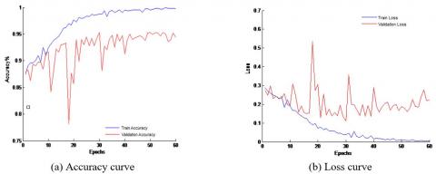
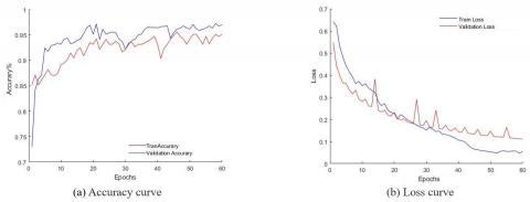
Relu is used as the activation function in the model's convolutional layer, and the output layer makes use of the binary classification-appropriate Sigmoid activation function. The model's test accuracy hits 0.952, and its ultimate training accuracy is 0.998. As can be observed, the binary categorization of plug seedling hole photos is a good fit for the model developed in this research. Classification recognition is supported by a compact model with only 9.5MB of parameter memory usage. Figure 6(a) shows that the training accuracy of the model continues to increase but the test accuracy starts to decrease as the model training iteration reaches the tenth iteration. The model appears to be overfitting at this point, and when the training iteration reaches the 40th iteration, the model starts to converge. It is clear that the model's rate of convergence is comparatively slow when Relu is used as the activation function. Figure 6(b) demonstrates that the accuracy rate curve and the model training loss curve have essentially the same trends. The training loss value decreases until it reaches its final value of 0.0056, and the verification loss also decreases until it reaches its final value of 0.2212, which has an increasing trend.4.2.3 Elu training results analysis.
Figure 6. Relu activation function model accuracy and loss curve
Figure 7. Elu activation function model accuracy and loss curve
The Elu activation function is used in the model's convolutional layer. Figure 7 shows that, while appearing to be overfit at the 10th training iteration, the model has converged by the 15th training iteration, which is consistent with the function's quick convergence speed. The model's final test accuracy is 0.938, training loss is 0, and test loss is 0.383. The model's final training accuracy is 1.0. Its ability to identify and categorize plug seedlings is marginally inferior to the Relu function. This paper chooses Relu and Elu as the activation functions of the convolutional layer, respectively, and conducts model regularization training and enhanced data set training in order to further investigate the impact of various activation functions on the recognition and classification capability of the model. These are the pertinent experiments:
5.2.3 Regularization training results analysis
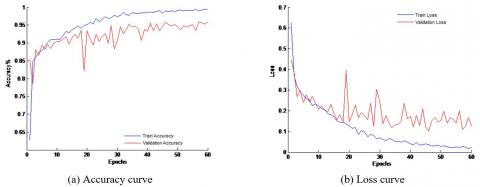
L2 regularization, Dropout regularization, Relu as the activation function of the convolutional layer, and Sigmoid as the activation function of the output layer are all used in the model, as seen in Figure 8. The training period's increasing trends for model test accuracy and loss value curves are essentially the same throughout, as can be seen in the figure, but after 20 training iterations, this upward trend starts to diverge from the training accuracy. The model's final test and training accuracy are both 0.993, along with the test and training loss of 0.0242 and 0.1236, respectively. The model's performance has increased in some ways. Elu is used as the activation function of the convolutional layer in Figure 9, Sigmoid is used as the activation function of the output layer, and the model uses L2regularization and Dropoutregularization. The upward trend of model test accuracy starts to lag behind the training accuracy once there are six training iterations. The two figures make it impossible to conclude that regularization can only partially address the model's overfitting issue.
Figure 8. Relu as an activation function for convolutional layers, Regularization model accuracy and loss curve
Figure 9. Elu as an activation function for convolutional layers, Regularization model accuracy and loss curve
5.2.4 Enhanced dataset training results analysis
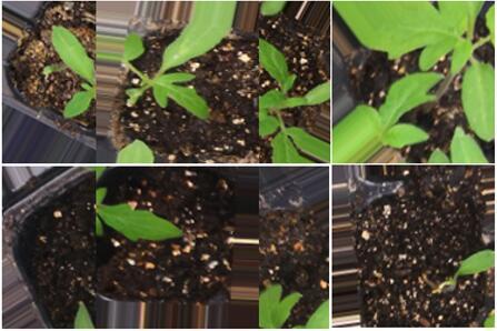
The model is trained with the enhanced data set. The hole images are randomly rotated, translated, and scaled at small angles to make the data set more representative. An example of the enhanced data set image is shown in Figure 10. The first row is the hole with seedlings, and the second line is the empty hole.
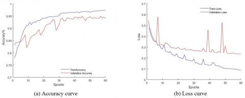
The training parameters were changed to train 200 photos per iteration because to the rise in the number of upgraded datasets. As seen in Figure 11, when the activation function of the convolutional layer adopts Relu, the overfitting problem of the model is solved and the final training accuracy of the model is 0.993, the test accuracy is 0.985, the training loss is 0.0099, and the test loss is 0.0233. Additionally, the change trend of the model training, test accuracy, and loss value curves are consistent in the entire training area. The model's performance has been considerably enhanced, and it can now accurately identify plug seedling holes in plugs. The accuracy rate curve and the loss value curve when training and verifying, respectively, have a significant difference when Elu is chosen as the activation function of the convolutional layer, as shown in Figure 12. Overfitting is still a problem, and the model's training accuracy is ultimately low. It is 0.9716, and the test accuracy is 0.9561, which is significantly less effective than Relu's classification effect as the convolutional layer's activation function. The two figures also show how rapidly the accuracy value can be increased and the loss value can be decreased when the Relu activation function is applied. Relu is therefore employed in this research as the convolutional layer's activation function.
Figure 10. Examples of Random Image Enhancement
Figure 11. Elu as an activation function for convolutional layers, Data enhancement model accuracy and loss curve
Figure 12. Elu as an activation function for convolutional layers, Data enhancement model accuracy and loss curve
In this study, a plug seedling device is designed, CNN is applied to the device's seedling recognition, and a plug seedling recognition model is created using the LeNet-5CNN model. The gathered plug seedling images are divided into individual hole images through image preprocessing, and large plug seedling image recognition is simplified into small hole image binary classification recognition. This significantly reduces the size of the recognition model and enhances the model's recognition accuracy. Relu is chosen as the activation function of the convolutional layer, Sigmoid is chosen as the activation function of the output layer, and the binary cross-entropy loss function is used to optimize the model. The method of data set enhancement is used to further improve the generalization ability of the model in order to solve the overfitting issue, and the result is that the recognition accuracy of the optimized model on the test set reaches 0.985. The issue of mutual interference between nearby hole seedlings is resolved by the CNNplug seedling recognition model developed in this paper. The model can fully suit the criteria of plug seedling devices due to its high identification accuracy and great generalizability, and intellect serves as a helpful guide.
This experiment does still have some flaws, though. For instance, the size of the data collection affects the model's dependability, and the paper's data set is rather tiny. To further raise the model's rate of recognition, more images will be added to the training set and the model will be modified in the following phase of the project.
This experiment does still have some flaws, though. For instance, the size of the data collection affects the model's dependability, and the paper's data set is rather tiny. To further raise the model's rate of recognition, more images will be added to the training set and the model will be modified in the following phase of the project.
This paper is supported by Open Fund of Chinese Academy of Sciences (Grant No.: 2020KFJJ14).
[1] Tai, Y.W., Ling, P.P., Ting, K.C. (1994). Machine vision assisted robotic seedling transplanting. Transactions of the ASAE, 37(2): 661-667. https://doi.org/10.13031/2013.28127
[2] Ryu, K.H., Kim, G., Han, J.S. (2001). Development of a robotic transplanter for bedding plants. Journal of Agricultural Engineering Research, 78(2): 141-146. https://doi.org/10.1006/jaer.2000.0656
[3] Wu, J.M., Zhang, X.C., Jin, X. (2015). Design and experiment on transplanter pot seedling disk conveying and positioning control system. Transactions of the Chinese Society of Agricultural Engineering, 2015(1): 47-52. https://doi.org/10.3969/j.issn.1002-6819.2015.01.007
[4] Jin, X. (2014). Study on automatic transplanting technology and device of vegetable pothole seedling. China Agricultural University.
[5] Feng, Q.C., Liu, X.N., Jiang, K., Fan, P.F., Wang, J. (2013). Devepment and experiment on system for tray-seedling on-line measurement based on line structured-light vision. Transactions of the Chinese Society of Agricultural Engineering, 2013(21): 143-149. https://doi.org/10.3969/j.issn.1002-6819.2013.21.018
[6] Jiang, H.Y., Shi, J.H., Ren, Y., Ying, Y.B. (2009). Application of machine vision on automatic seedling transplanting. Transactions of the Chinese Society of Agricultural Engineering, 2009(5): 127-131. https://doi.org/10.3969/j.issn.1002-6819.2009.05.24
[7] Wang, Y.W., Xiao, X.Z., Liang, X.F., Wang, J., Wu, C.Y., Xu, J.K. (2018). Plug hole positioning and seedling shortage detecting system on automatic seedling supplementing test-bed for vegetable plug seedlings. Transactions of the Chinese Society of Agricultural Engineering, 2018(12): 35-41. https://doi.org/10.11975/j.issn.1002-6819.2018.12.005
[8] Zhang, Z.B., Luo, X.W., Zang, Y., Hou, F.X., Xu, X.D. (2011). Segmentation algorithm based on color feature for green crop plants. Transactions of the Chinese Society of Agricultural Engineering, 2011(7): 183-189. https://doi.org/10.3969/j.issn.1002-6819.2011.07.032
[9] LeCun, Y., Bengio, Y. (1995). Convolutional networks for images, speech, and time series. The handbook of Brain Theory and Neural Networks, 3361(10): 1995.
[10] Wang, C., Wu, X.H., Li, Z.W. (2018). Extraction of multi-scale hierarchical features to identify maize weeds based on convolutional neural network. Transactions of the Chinese Society of Agricultural Engineering, 2018(5): 144-151. https://doi.org/10.11975/j.issn.1002-6819.2018.05.019
[11] Ma, J.C., Du, K.M., Zheng, F.X., Zhang, L.X. Sun, Z.F. (2018). Recognition system of greenhouse cucumber disease based on convolutional neural network. Transactions of the Chinese Society of Agricultural Engineering, 2018(12): 186-192.
[12] Brahimi, M., Boukhalfa, K., Moussaoui, A. (2017). Deep learning for tomato diseases: classification and symptoms visualization. Applied Artificial Intelligence, 31(4): 299-315. https://doi.org/10.1080/08839514.2017.1315516
[13] Yang, Z.Y., Zhang, W.Q., Li, W., Chen, Y. (2014). Adjustment method of leaf orientation of transplanting pot seedlings based on monocular vision. Transactions of the Chinese Society of Agricultural Engineering, 2014(14): 26-33. https://doi.org/10.3969/j.issn.1002-6819.2014.14.004
[14] Krizhevsky, A., Sutskever, I., Hinton, G.E. (2017). Imagenet classification with deep convolutional neural networks. Communications of the ACM, 60(6): 84-90. https://doi.org/10.1145/3065386
[15] Goodfellow I, Beggio Y, Courville A. (2016). Deep learning. Book in preparation for MIT Press.
[16] Lin, Z.L., Wang, C.L., Hu, Y.J., Zhang, Y. (2018). Convolution neural network model for SAR image target recognition. Chinese Journal of Image and Graphics, 23(11): 1733-1741.
[17] Glorot, X., Bordes, A., Bengio, Y. (2011). Deep sparse rectifier neural networks. In Proceedings of the Fourteenth International Conference on Artificial Intelligence and Statistics, pp. 315-323.
[18] Srivastava, N., Hinton, G., Krizhevsky, A., Sutskever, I., Salakhutdinov, R. (2014). Dropout: A simple way to prevent neural networks from overfitting. The Journal of Machine Learning Research, 15(1): 1929-1958.
[19] De Boer, P.T., Kroese, D.P., Mannor, S., Rubinstein, R.Y. (2005). A tutorial on the cross-entropy method. Annals of Operations Research, 134(1): 19-67. https://doi.org/10.1007/s10479-005-5724-z
[20] LeCun, Y., Bottou, L., Bengio, Y., Haffner, P. (1998). Gradient-based learning applied to document recognition. Proceedings of the IEEE, 86(11): 2278-2324. https://doi.org/10.1109/5.726791
[21] Hinton G. (2012). Rmsprop: Divide the gradient by a running average of its recent magnitude. Neural networks for machine learning, Coursera lecture 6e.