Shaila Chugh* | Sachin Goyal | Anjana Pandey | Sunil Joshi
© 2022 IIETA. This article is published by IIETA and is licensed under the CC BY 4.0 license (http://creativecommons.org/licenses/by/4.0/).
OPEN ACCESS
Breast cancer is a leading cause of death among women. The death rate is reduced when this disease is detected early with the help of mammography. Deep learning is a method that radiologists use and request to help them make more accurate diagnoses and enhance their outcome predictions. This work presents a novel strategy comprising a pre-processing method and a mix of morphological and multi-thresholding using Otsu's technique based segmentation technique, which was tested on the Mini-MIAS dataset of 322 images. For Speed-Up Robust Features (SURF) selection, the inbuilt feature extraction is done utilizing multiple colour and texture features approaches. At the classification level, a new layer is added that performs 70 percent training and 30 percent testing of the deep neural network. There are two primary steps in the training phase: (1) Develop a model for dividing breast tissue into dense and non-dense categories. (2) Develop a model for classifying breast regions into mass and non-mass. The results show that the accuracy rate of the proposed automated DL approach is higher than that of other state-of-the-art models. The average accuracy (ACC) rates of the three types of cancer, i.e., normal, benign, and malignant cancer, utilizing the suggested method are 91 percent, 94 percent, and 93 percent, respectively, according to experimental results.
Otsu’s technique, neural network, MIAS, morphological operation, deep learning
Breast cancer is a leading cause of death among women. Breast cancer is a leading cause of death among women. The death rate is reduced when this disease is detected early with the help of mammography. It becomes more difficult for radiologists to finish the diagnostic process in the short time provided as the number of patient increases. The goal of this research is to use deep learning to assist radiologists in enhancing the rate of prompt and accurate breast cancer detection (DL). Deep learning (DL) is a method that radiologists use and request to help them make more accurate diagnoses and enhance their outcome predictions.
The classification of breast cancer is greatly aided by machine learning (ML). The various ML based diagnosis techniques that have been proposed in literatures. ML is a subset of artificial intelligence. Many developers use machine learning to retrain their existing models, which helps them perform better. Machine learning is used for linear data. When the amount of data is small, machine learning provides superior results; but, when the amount of data is large, it does not. Three distinct machine learning techniques are used to train the model. Supervised machine learning works on known data with the assistance of a supervisor. Without any supervision, unsupervised machine learning is used. Reinforcement machine learning is becoming less popular. These algorithms use the best information from previous knowledge to make the best decisions.
Deep learning is a branch of machine learning. It is a type of unsupervised learning that learns from data. The information may not be labeled or be structured properly. A deep network is one that has more than two hidden layers in a deep neural network. The input layer is on the top layer, and the output layer is on the bottom layer. The hidden layer, which is the intermediate layer, has more layers than a neural network. A node called neurons houses the layer. Deep learning is distinct from machine learning in that it advances you toward your objective more quickly.
Although the concept of classification algorithms is gaining traction in studies for breast cancer detection and diagnosis, radiologists still confront gaps and problems. Missing training data, a limited live dataset, machine learning methodologies on short datasets, and other challenges will be addressed by constructing a Deep NN model that works for tiny datasets. DNN has an advantage over machine learning in that it has a greater detection accuracy than ML models and helps radiologists diagnose worrisome lesions more precisely by providing quantitative data. According to a recent study, adopting DL techniques reduces human mistake rates for breast cancer diagnoses by 85%. The current generation of DNN models is made to help radiologists discover even the tiniest breast tumours in their very early stages, alerting the radiologist to the need for additional investigation.
This study presents a novel methodology comprising a pre-processing method, multilevel thresholding image segmentation, integrated feature extraction for Speed-Up Robust Features (SURF) selection, and deep NN based classification, which was tested on the Mini-MIAS dataset of 322 images.
In this paper the combination of morphological operation and mult-thresholding using Otsu’s technique for breast tissue segmentation is suggested that identifies the weakness of unidirectional recognition by allowing recognition rates to exceed 85 percent and more, which significantly enhances the accuracy. Apart from these, segmentation of the breast tissues is achieved properly, if we have good quality image. So, enhancing the quality of image became the essential step in segmentation. In this paper, we have applied preprocessing step for noise handling, resizing, and contrast enhancement of image.
The existing work is explained in details in section 2. The suggested methodology is described in Section 3, and the proposed workflow and validation process is discussed in Section 4. The 5th section summarizes the findings and suggests future research.
This section outline previous research in the field that is relevant to the current study. Breast cancer can be detected using one of two approaches. Machine learning comes first, followed by deep learning.
Rathi and Pareek [1] suggested a model based on a hybrid method using machine learning and extrapolated from ROI 20 texture features. In order to get the best results, it used four classifiers and the MRMR feature selection algorithm. SVM, Nave Bays, Function trees, and End Meta were all utilized by the author, and the results were compared. SVM was found to be an effective classifier. Another machine learning-based hybrid approach was presented by Tahmooresi et al. [2] to discover superior outcomes.
Aslan et al. [3] proposed a machine learning approach, but they utilized a different classifier. Extreme Learning Machine, SVM, KNN i, and ANN were the classifiers employed by the author. To get better results, the classifier was tweaked a little. So far, the results show that the Extreme Learning Machine is the winner.
Shravya et al. [4] suggested a paradigm for supervised machine learning. Classifiers including Logistic Regression, SVM, and KNN were used in this study. The dataset was obtained from the UCI repository, and the findings were evaluated in light of their overall performance. This shows that SVM was an effective classifier on the Python platform, with an accuracy rate of 92.7%.
SVM classifier was used to examine the performance of the ANN model developed by Wadkar et al. [5]. According to the author, ANN had a 97% accuracy rate and SVM had a 90% accuracy rate. Without SVM, the accuracy was improved, according to the author.
Dheeba et al. [6] use a Particle Swarm Optimized Wavelet Neural Network to identify and diagnose breast cancer (PSOWNN). Subashini and Jeyanthi [7] advocated using ultrasound scans to identify breast cancer. They eliminated noise with DWT, segmented with an active contour model, and classified with a back propagation neural network. S. A research by Antony and Ravi [8] suggests using histogram equalization to improve image quality. When calculating volumetric values, data from the intensity characteristics is gathered and then processed. K-means clustering technique is used for categorization. The Gabor filter is used to reduce noise. There are two databases used in this analysis: MIAS and DDSM. Classification accuracy of at least 99 percent is required. The CAD (computer-aided diagnostic) system was defined by Radovic et al. [9] For the detection of normal and abnormal breast patterns. They compared the categorization results using seven different classifiers. DWT was employed to narrow the scope of the study (ROI).
de Oliveira Martins et al. [10] described K-means and co-occurrence matrix in 2009 and utilized SVM classifier to detect the masses. Images are divided into masses and non-masses for classification based on shape and texture descriptors.
For a huge collection of mammography images, Anjaiah et al. [11] presented multi-ROI segmentation. It substantially aids in the discovery of the best textural features in mammography pictures. Existing ROI segmentation does segmentation without knowledge of the mammography model's universal shape. For generating the universal shape (or average model parameters) of mammograms, the proposed multi-ROI segmentation utilized a huge collection of mammograms. It aids in obtaining accurate texture or form aspects of a suspected mammography for the identification of breast cancer.
A wide spectrum of investigations employs machine learning. Machine learning techniques, on the other hand, have some flaws that deep learning addresses. Several researches have used CNNs to perform mammogram-related tasks, such as breast lesion detection, benign and malignant breast mass classification, micro-calcification recognition, and combinations of these tasks.
Fonseca et al. used CNNs to extract features from mammograms and a support vector machine classifier to do density classification [12]. With the use of three extra generated images, Ahn et al. constructed a CNN architecture to classify the input mammography patches into dense or fatty tissues, and estimate the mammographic density by aggregating the findings of all patches [13]. Based on a sliding window segmentation methodology, Li et al. developed a similar method to classify mammographic density [14]. As a reference for these two experiments, manual segmentation maps of dense regions are required.
The Man and Machine Mammography Oracle (MAMMO), a clinical decision support system that can split mammograms into those that can be safely classified by a machine and those that cannot, requiring a radiologist's interpretation, was created by Kyono et al. [15]. The initial part of MAMMO is a special multi-view convolutional neural network (CNN with multi-task learning (MTL). The second part of MAMMO is a triage network, which selects which mammograms the CNN can accurately and reliably diagnose and which mammograms need to be evaluated by a radiologist using the radiological evaluation and diagnostic predictions of the first network's MTL outputs as input.
Zhang et al. [16] proposed using CNNs to classify mammograms and tom synthesis images. They analyzed data from 3000 mammograms and tom synthesis scans. Different CNN models were developed to identify both 2-D and 3-D mammograms, and each classifier was evaluated using truth-values obtained by histology results from the biopsy and two-year negative mammography follow-up confirmed by professional radiologists. They have developed and optimized a system that used transfer learning and data augmentation to diagnose breast cancer automatically using mammograms and tom synthesis data.
Shen et al. [17] construct a deep learning algorithm that can accurately detect breast cancer on screening mammograms using a "end-to-end" training technique that efficiently leverages training datasets with either comprehensive clinical annotation or just the cancer status (label) of the entire image. Lesion annotations are only required during the initial training stage; subsequent stages only require image-level labels, eliminating the need for difficult-to-access lesion annotations. Our-all convolutional network method for classifying screening mammograms outperformed previous methods.
Tardy et al. [18] suggested a model to solve the challenge of evaluating breast density as an image wise regression task with the goal of quantifying the percentage of fibro glandular tissue. Their method is based on deep learning, and it provides a clinically acceptable estimate with few expert annotations. They also talk about using the X-ray acquisition parameters as a source of additional information for the neural network.
Shen et al. [19] present a mixed-supervision guided technique and a residual-aided ii classification U-Net model for joint segmentation and benign-malignant classification (ResCU-Net). By coupling strong supervision in the form of a segmentation mask and weak supervision in the form of a benign-malignant label via a simple annotation procedure, their method efficiently segments tumour regions while simultaneously predicting a discriminative map for identifying benign-malignant tumour types.
Wang et al. [20] use pre-trained deep convolution neural networks (DCNNs) to create a multi-network feature extraction model, design an effective feature dimension reduction strategy, and train an ensemble support ii vector machine (E-SVM). First, they use scale transformation and colour enhancement algorithms to preprocess the histology pictures. Second, four pre-trained DCNNs are used to extract multi-network characteristics (e.g., DenseNet-121, ResNet-50, multi-level InceptionV3, and multi-level VGG-16). Third, for performance enhancement and over fitting reduction, a feature selection approach based on dual-network orthogonal low-rank learning (DOLL) is devised. Finally, an E-SVM is trained to execute the classification task using fused features and a voting technique, classifying the photos into four categories (i.e., benign, in situ carcinomas, invasive carcinomas, and normal).
Song et al. [21] propose a new combined feature CAD approach based on DL for categorizing mammographic masses into three categories: normal, benign, and cancerous (malignant). The Deep Convolution Neural Network (DCNN) was used as a feature extractor to score three different types of breast masses. The score features and picture texture features are then merged as input to the classifier. This information was extracted from mammograms using these characteristics, and the Support Vector Machine (SVM) and Extreme Gradient Boosting (XGBoost) classifiers were trained for the classification job. Although Faster R-CNN has been employed in medical imaging, there is a paucity of material in the field of breast imaging.
Ribli et al. [22] used the DDSM database of 2620 scanned -film mammograms to train a Faster R-CNN model, which they subsequently tested against the INbreast dataset of malignant tumours. To solve the problem of excessive class imbalance between the foreground and background, Jung et al. [23] suggested a mass detection model based on RetinaNet [24] and a new loss function dubbed focused loss. The network's performance was assessed using both a private (GURO) and a public (INbreast) dataset. Morrel et al. [25] proposed a neural network based on deformable convolutional nets and a region-based fully convolutional network (R-FCN) [26]. Despite the fact that the network was trained with the OPTIMAM Mammography Image Database (OMI-DB) [27], the findings were only made available for the DREAMS challenge competitive phase [28].
In Full-Field Digital Mammograms, Agrawal et al. [29] provide a fully automated method for detecting masses (FFDM). The Faster-RCNN model was employed in their technique, which was used to detect masses in the large-scale OPTIMAM Mammography Image Database (OMI-DB). The Faster R-CNN model, which was trained on Hologic images, uses transfer learning to detect masses in smaller databases containing FFDMs from the GE scanner and another public dataset INbreast (Siemens scanner).
Training a deep CNN model with a limited amount of medical data is difficult, but transfer learning (TL) and augmentation techniques can help. According to the literature, heterogeneous breast densities make masses more difficult to detect and classify than calcifications. Although DL methods show promising improvements in breast cancer diagnosis, there are still issues of accuracy, data scarcity, and computational cost, which have been significantly mitigated by data augmentation and improved computational power of DL algorithms.
In our method to achieve higher accuracy on small dataset, in place of data augmentation, we have created three separate DL models: one model for dividing breast tissue into dense and non-dense categories and another two models for classifying breast regions into mass and non-mass based on dense and non-dense dataset.
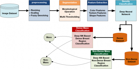
This section introduces our devised methodology, which was trained and evaluated on the MIAS datasets [30]. MIAS consists of 322 mammography images with a resolution of 1024 x 1024 pixels. All images are in portable grey map format (.pgm). As a partial resolution of 0.05 mm pixels and 2 bit density, SCANDIG-3 is used to digitalize them. Mass, micro-calcification, architectural distortion and bilateral asymmetry are among the abnormalities visible in these images. On the basis of density, the MIAS dataset can be classified as either dense or fatty. Among the 322 images, 207 mammograms are normal, 63 benign mammograms, and 52 malignant mammograms. Malignant cancer is the most well-known type of breast cancer disease, and it is the leading cause of death in women. We will now go over the various subsections (see Figure 1) of the suggested method one by one.
3.1 Image preprocessing
Before being fed into the NN model, images are preprocessed with resizing, scaling, picture denoising, and contrast enhancement techniques. A combination of mean and median filter is used to remove digitalized noise. Proposed Fuzzy filtering is utilized for enhancing the contrast of the image.
3.2 Image denoising based on mean-median filter
Filtering is a technique for removing unwanted information from an image by perception and making it more suitable for the next step in image processing. To remove speckle sounds from photos, various types of filtration are used. The image was de-specked using a mean-median filter in this investigation. The image before and after applying the mean-median filter is shown in Figure 2(b) and 2(b), respectively.
Figure 1. Proposed methodology
|
(a) |
(b) |
Figure 2. (a) Input image (b) denoised image after mean- median filter
3.3 Fuzzy based contrast enhancement
Denoising the input image is followed by applying the proposed fuzzy contrast enhancement phase, which improves the mammography image further. Three steps make up the proposed fuzzy phase. In the first phase, image which is in the spatial domain is converted into fuzzy domain. In the next phase, fuzzification is applied on the image which is in fuzzy domain. S-membership function is used that updates the pixels values according to the condition. Finally in third phase, defuzzification is applied on updated fuzzy image which convert the contrast enhanced fuzzy image back to the spatial image. For overexposed and underexposed sections, the image's grey levels are well-known to be quite close to the image's maximum grey level and minimum grey level. To make the contrast enhancement more adaptive and more effective and to avoid over-enhancement/under-enhancement, adaptive fuzzy contrast enhancement is applied. The advantage of proposed fuzzy phase is that it boosts the contrast of image locally, rather than boosting the contrast globally.
3.3.1 Image in fuzzy set notation
The initial image xi,j of size M x N with intensity levels in the range of [0 L-1] can be considered an array of fuzzy singletons in the fuzzy set notation. The degree of brightness of the grey level is represented by the membership value for each element in this array. In fuzzy set notation, we can write:
$X=\cup\left\{\mu\left(x_{i, j}\right)\right\}=\left\{\frac{\mu_{i, j}}{x_{i, j}}\right\}$
$i=1,2, \ldots, M$ and $j=1,2, \ldots, N$ (1)
where, $\mu\left(x_{i, j}\right)$ denotes the degree of brightness possessed by the gray level intensity of the (i,j) th pixel.
3.3.2 Fuzzification
A fuzzy set's fuzziness is described by its membership function. A fuzzy set's membership function converts all of the set's elements to real values between 0 and 1. For a gray level image, the S-function is the most widely employed membership function.
$\mu\left(x_{i j}\right)=\left\{\begin{array}{lr}0 & \text { for } x_{i j} \leq a \\ \frac{x_{i j}-a}{(b-a)(c-a)} & \text { for } \mathrm{a}<x_{i j} \leq \mathrm{b} \\ 1-\frac{\left(x_{i j}-c\right)^2}{(c-b)(c-a)} & \text { for } \mathrm{b}<x_{i j} \leq \mathrm{c} \\ 1 & \text { for } x_{i j} \geq c\end{array}\right.$ (2)
where, xi,j is the image's intensity, and a, b, and c are the S-shape-determining function's parameters. The parameters a, b, and c are calculated as follows:
•Assume that the image has a range of gray scale values from Lmin to Lmax.
•Divide the image into 16*16 sub images.
•Calculate the histogram of each sub images as H1, H2, ..., Hk.
Determine the height of each histogram i.e., M1, M2, ..., Mk, where $M_i=\max \left(H_i\right)$.
•Calculate the average height of the local maxima.
$\bar{H}=\frac{1}{k} \sum_{i=1}^k M_i$ (3)
•If the height of a local maximum is more than the average height, $P_i=H_i$, if $H_i \geq \bar{H}$ choose it as a peak; otherwise, ignore it.
•Select the grey level of the first peak P1 and the last peak Pk, that is, a=P1 and c=Pk, to determine the value of parameter a and c.
•Determine the midpoint of the interval [a,c] as parameters b.
•The image intensity levels converted from the spatial domain to the fuzzy domain using the calculated membership function.
3.3.3 Defuzzification
Defuzzification is used to change the membership value from the black to grey level, making the contrast enhancement more adaptive and effective while avoiding over- or under-enhancing. The following formula is used to transforms the membership value $\mu\left(x_{i j}\right)$ to the gray level:
${{X}_{ij}}^{'}=\left\{ \begin{align}& {{L}_{\min }} \\ & \mu ({{X}_{ij}})=0 \\& {{L}_{\min }}+\frac{{{L}_{\min }}-{{L}_{\max }}}{c-a}\sqrt{\mu ({{X}_{ij}})(b-a)(c-a)}\text{ } \\& 0<\mu ({{X}_{ij}})\le \frac{(b-a)}{(c-a)} \\ & {{L}_{\min }}+\frac{{{L}_{\min }}-{{L}_{\max }}}{c-a}(c-a-\sqrt{1-\mu ({{X}_{ij}})(b-a)(c-a))} \\ & \frac{(b-a)}{(c-a)}<\mu ({{X}_{ij}})<1 \\& {{L}_{\max }} \\& \mu ({{X}_{ij}})=1 \\ \end{align} \right.$ (4)
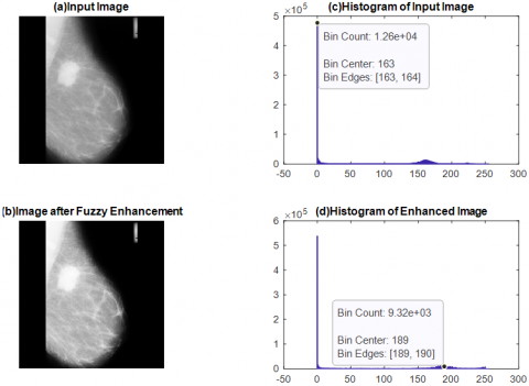
It's well-known that the image's grey levels skew toward the extremes of the image's overexposed and underexposed regions, respectively. Figure 3 depicts the final outcome following the use of fuzzy phases.
Figure 3. Image after fuzzy enhancement
3.4 Breast tissue segmentation based on morphological operation and multi thresholding
Mammogram Image segmentation step is divided into two steps: Morphological based exacting breast tissue component operation containing shapes of interest and second one is Otsu’s based segmentation of breast tissue.
3.4.1 Morphological operation based extraction of shapes of interest
Morphological image processing (or morphology i) refers to a class of image processing algorithms that deal with the shape of picture features. Typically, morphological treatments are used to eliminate flaws introduced during segmentation.
Dilation and erosion are the two most important morphological activities. Dilation allows items to extend, potentially filling in small gaps and linking disparate objects. Erosion causes items to diminish by etching away (eroding) their boundaries. These operations can be tailored to a specific application by selecting the structuring element (a rectangular array of pixels with the values 1 or 0), which controls how the objects will be dilated or eroded [9].
Morphological algorithms have been utilized for pre- or post-processing photos containing shapes of interest, in addition to providing useful tools for extracting image components. Morphological processes strike objects with structuring elements and reduce them to disclosing shape. It's used to extract picture elements like skeletons, borders, and the convex hull. Erosion and dilation are two common morphological activities. Erosion is the process by which features in an image are disconnected and removed. Erosion is seen as a filtering operation. It is denoted by the symbol $1 \Theta$ and written as
$A\Theta B=\{z|{{(B)}_{z}}\bigcap {{A}^{c}}=\phi \}$ (5)
Dilation is the process of connecting the features in an image. The dilation procedure is regarded as a reconstructive procedure. It is denoted by the symbol $\oplus$ and formulated as
$A\oplus B=\{z|{{(B)}_{z}}\bigcap A\ne \phi \}$ (6)
The opening and closing operations of morphology is built upon erosion and dilation. The basic neighborhood structure linked with morphological image processing serves as the underlying framework. Morphological operators can be applied to images based on the shape and size of a morphological matrix. It is also called as mask or kernel. Structuring element matrix has 0 values to represent black and 1 value to represent white. The design of structuring element, their shape and size, is crucial to the success of the morphological operations that use them.
Figure 4 shows the output after applying morphological operation.
|
(a) |
(b) |
Figure 4. Image after morphological operation
3.4.2 Image segmentation based on multithresholding
To distinguish malignant objects from normal images, image segmentation is used. Multilevel thresholding utilizing the Otsu method is used for image segmentation where the image is divided into three levels using IM Quantize with two threshold levels.
Otsu's approach is a global thresholding method that Otsu proposed [31]. The appropriate threshold is set automatically and consistently using this method, which is based on the histogram's global attribute.
Let L be the total number of grey levels in the image. The pixels then have a grey level range of 0 to L-1. Let's call the number of pixels at level by ni. Assume that a threshold k is determined, with C1 consisting of pixels with levels [0, 1, 2, ..., k] and C2 consisting of pixels with levels [k+1, ..., L-1]. The Otsu technique determines the best k threshold value to maximize the variation across classes, which is defined as
$\sigma _{B}^{2}(k)={{P}_{1}}(k){{[{{m}_{1}}(k)-{{m}_{G}}]}^{2}}+{{P}_{2}}(k){{[{{m}_{2}}(k)-{{m}_{G}}]}^{2}}$ (7)
The Probability P1(k) that a pixel is assigned to class C1 is given by:
${{P}_{1}}(k)=\sum\limits_{i=0}^{k}{{{p}_{i}}}$ (8)
Similarly, the probability of pixels assigned to class C2 is defined as:
${{P}_{2}}(k)=\sum\limits_{i=k+1}^{L-1}{{{p}_{i}}=1-{{P}_{1}}(k)}$ (9)
The Global mean mG is defined as:
${{m}_{G}}=\sum\limits_{i=0}^{L-1}{i{{p}_{i}}}$ (10)
The mean intensity for class C1 is given by
$m(k)=\sum\limits_{i=0}^{k}{i{{p}_{i}}}$ (11)
The between class variance is given by
$\sigma _{B}^{2}(k)=\frac{{{[{{m}_{G}}{{P}_{1}}(k)-m(k)]}^{2}}}{{{P}_{1}}(k){{[1-{{P}_{1}}(k)]}^{2}}}$ (12)
The optimal threshold value k is selected from largest value of $\sigma_B^2(k)$. The ratio of the between class variance to the total image intensity variance,
$\eta (k)=\frac{\sigma _{B}^{2}(k)}{\sigma _{G}^{2}}$ (13)
Is a measure of reparability of image intensities into two classes (foreground and background) which can be shown to be in range 0≤η (k*) ≤ 1. Where k* is the optimal threshold.
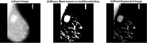
After Applying Global Thresholding Using Otsu Method on the image getting from previous step is shown if Figure 5.
3.5 Feature extraction
We extract unique characteristics from the breast cancer image. The 2D Wavelet Transform will be used to extract features. Entropy, Mean, Mean Absolute Deviation, Median Absolute Deviation, Energy, Standard deviation, L1 norm, L2 norm, Kurtosis, and Skewness are all features derived using the wavelet technique. Contrast, Correlation, Energy, and Homogeneity are the texture features extracted by GLCM.
Color, texture, shape, morphology, and other aspects of the object are the major features from which we may recognize disease effectively [32]. In this article, we've chosen a few of these traits for disease detection. Some of the picture feature formulas are shown in Table 1.
Figure 5. Segmented image after applying Ostu’s method
|
(a) input images |
(b) images applied mean filter and fuzzy denoisng filter |
|
(c) images with segmented regions by morphological and Otsu’s method |
(d) color and texture feature extracted |
Figure 6. Segmentation and feature extraction steps
Table 1. Image features
|
SN |
Color Feature |
Formula |
|
1 |
Energy |
${{f}_{1}}={{\sum\limits_{i}{\sum\limits_{j}{\left\{ p(i,j) \right\}}}}^{2}}$ |
|
2 |
Contrast |
${{f}_{2}}\,=\sum\limits_{i}{\sum\limits_{j}{{{\left| i-j \right|}^{2}}}}p(i,j)$ |
|
3 |
Correlation (1): |
${{f}_{3}}\,=\sum\limits_{i}{\sum\limits_{j}{\frac{\left( i-{{\mu }_{i}} \right)\left( j-{{\mu }_{j}} \right)p(i,j)}{{{\sigma }_{i\,}}{{\sigma }_{j}}}}}$ |
|
4 |
Correlation (2): |
${{f}_{4}}\,=\frac{\sum\nolimits_{i}{\sum\nolimits_{j}{(i,j)\,p(i,j)-{{\mu }_{x\,}}{{\mu }_{y}}}}}{{{\sigma }_{x\,}}{{\sigma }_{y}}}$ |
|
5 |
Homogeneity: |
${{f}_{5}}\,=\sum\limits_{i}{\sum\limits_{j}{\frac{p(i,j)}{1+\left| i-j \right|}}}$ |
|
6 |
Maximum Probability: |
${{f}_{6}}\,=\max (p(i,j))$ |
|
7 |
Sum of Squares Variance |
${{f}_{7}}\,=\sum\limits_{i}{\sum\limits_{j}{{{(i-\mu )}^{2}}p(i,j)}}$ |
|
8 |
Inverse Difference Moment |
${{f}_{8}}\,=\sum\limits_{i}{\sum\limits_{j}{\frac{1}{1+{{(i-j)}^{2}}}}}p(i,j)$ |
|
9 |
Sum Average |
${{f}_{9}}\,=\sum\limits_{i=2}^{2{{N}_{g}}}{i{{p}_{x+y}}(i)}$ |
|
10 |
Sum Variance |
${{f}_{10}}\,=\sum\limits_{i=2}^{2{{N}_{g}}}{{{(i-{{f}_{8}})}^{2}}{{p}_{x+y}}(i)}$ |
|
11 |
Sum Entropy |
${{f}_{11}}\,=-\sum\limits_{i=2}^{2{{N}_{g}}}{{{p}_{x+y}}(i)\,\log \{{{p}_{x+y}}(i)\}}$ |
|
12 |
Entropy |
${{f}_{12}}\,=-\sum\limits_{i}{\sum\limits_{j}{p(i,j)\log \{p(i,j)\}}}$ |
|
13 |
Difference Variance |
f13= variance of p(x-y) |
|
14 |
Difference Entropy |
${{f}_{14}}\,=-\sum\limits_{i=0}^{{{N}_{g}}-1}{{{p}_{x-y}}(i)\,\log \{{{p}_{x-y}}(i)\}}$ |
|
15 |
Information Measures of correlation |
${{f}_{15}}\,=\frac{HXY-HXY1}{\max \{HX,HY\}}$ |
where are the means and standard deviations of and p(i, j) is the distribution probability of gray level difference between adjacent pixels.
The complete process of getting the feature extracted from the input image can be viewed by the Figure 6.
3.6 Normalization
Normalization is a technique for scaling in which value is shifted and resized between 0-1. It is also known as Min-Max scaling. Here is the normalization formula:
${X}'=\frac{X-{{X}_{\min }}}{{{X}_{\max }}-{{X}_{\min }}}$ (14)
Scaling turns features with various scales into a fixed scale from 0 to 1. This guarantees that the specific feature does not dominate other features.
3.7 Density classification model
The next stage is to construct a model that categorizes breasts based on density, because masses in non-dense breasts often have a high density that can be confused with healthy tissue in dense breasts, making it impossible to identify masses in different types of breasts with a single model. This was done with the help of a multi-layered deep neural network. Digital Database for Screening Mammography (DDSM) data contains dense and non-dense breast images that are loaded into a multi-layer deep neural network for classification and detection training.
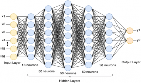
The back-propagation approach was used with MATLAB's Neural Network Pattern Recognition Tool to accomplish the density classification analysis (NPRT). The suggested neural networks are made up of one input layer with 16 neurons for each feature vector, five hidden layers, and one output layer with two neurons for each dense/non-dense class. The network extracts and categorizes patterns from the features that have been extracted. Each layer's output is used as input for the next [27, 28]. The suggested deep neural network's architecture is shown in Figure 7.
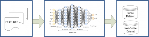
In order to train the network, scaled conjugate gradient back propagation is used. The network's input is the extracted colour and texture features, while the target data is the image class label. The network's performance may be observed through the training window, and if the error is too high, the network is retrained to produce more precise and efficient results. Finally, the images are given a class and inserted into the appropriate database. Figure 8 depicts the entire classification process.
Figure 7. Proposed feed forward back propagation neural network
Figure 8. The process of classification based on dense and non-dense regions
3.8 Regions classification models
By using the density model created in the preceding phase, a dataset based on image density can be constructed. This step is to develop models for distinguishing between dense and non-dense breast lumps. The DNN will be used to select candidates for the creation of models that classify breast regions into masses and non-masses.
We separate the dense and non-dense breasts datasets from the training images using the DDSM's marking file. There will now be two models constructed, one for dense breasts and the other for non-dense breasts, for the classification of regions.
A DNN is used to generate two classification models for the images once the dense breasts and the non-dense breasts have been separated. This stage uses the same DNN architecture as the density model, which has one input, five hidden layers, and one output layer: At this point (and in the training phase), there are three models: one for density classification, one for the classification of masses and non-masses for dense breasts, and one for the mass classification in non-dense breasts. On a test base, these models will be used to determine breast density and segmentation.
Here we'll go through the models created during the methodology's training phase and the outcomes that were obtained during the testing phase.
4.1 Dataset
The proposed algorithm will be tested on all 322 MIAS sample images. A total of 322 1024 x 1024 pixel mammography pictures are included in the MIAS. All of the images are in a format that is easy to move around. They are all in grey map format (.pgm). These images are digitized using SCANDIG-3, which provides 2 bit density resolution and partial resolution of the 0.05 mm pixels. These images show a variety of anomalies, including mass, micro- calcification, architectural distortion, and bilateral asymmetry. The MIAS dataset can be categorized as fatty, fatty glandular, or dense glandular based on density. In the 322 pictures, 207 are normal, 63 are benign, and 52 are malignant. These photos were split into two sets: one for training and the other for testing purposes. This was done in such a way that identical patient pairs were guaranteed to be in the same base. A 3.2 GHz processor and 4 GB of RAM will be used for simulations.
4.2 The quality parameters
Confusion matrix, ROC curve with AUC score, and correlation coefficient are used to evaluate the suggested algorithm's performance. A confusion matrix is a table that contains information about the proposed method's predicted and actual class. Tables 2 and 3 show the confusion matrix for two classes (benign and malignant) as well as performance measures.
Table 2. Confusion matrix
|
Actual class |
Predicted class |
|
|
Positive |
Negative |
|
|
Positive |
TP (true positive) |
FN (false negative) |
|
Negative |
FP (false positive) |
TN (true negative) |
Table 3. Performance parameter
|
Measure |
Definition |
|
TPR or recall |
TP / (TP + FN) |
|
FPR |
FP / (FP + TN) |
|
precision |
TP / (TP + FP) |
|
ACC |
(TP + TN/K) |
The TPR (true positive rate) and the FPR (false positive rate) are two key performance indicators. Out of the total number of malignant ROIs, the TPR estimates the percentage of malignant ROIs that are correctly diagnosed. Out of the total number of benign ROIs, the FPR parameter determines the number of benign ROIs that were wrongly classified. In the evaluation of binary classification quality, the F-measure and MCC are crucial. The F-measure is calculated as the harmonic mean of the terms 'precision' and ‘recall’, and is equal to
$F-measure=\frac{2\times recall\times precision}{recall+precision}$ (15)
4.3 Density classification evaluation
To construct dense models, photos are preprocessed, segmented, and feature selected. Following that, we get models that can classify dense and non-dense breasts. We utilized 1000 epochs as a stopping condition for training the density model, with a learning rate of 0.005, a batch of 16 features, and a validation rate of 15%.
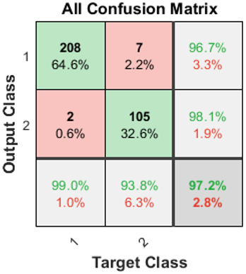
Table 4 shows the confusion matrix of the proposed dense model that classifies the breasts into mass or non-mass. Out of the 210 non dense breasts, out model accurately identify 208 non-dense breasts and out of the 113 dense breasts, out model accurately identify 105 dense breasts. Seven dense breasts are wrongly classified as non-dense breast. Similarly, 2 non-dense images are wrongly classified as dense breast.
Results of the validation metrics such as Accuracy, Sensitivity, Specificity and Precision of proposed dense models are shown in Table 5. Accuracy of the proposed method is 97.2% This shows that the models are able to detect the dense regions accurately. Sensitivity, Specificity and Precision values for the non-dense and dense breast are 99.0, 93.8, 96.7 and 93.8, 99.0, 98.1, respectively, which shows the outperform of the proposed models.
Table 4. Confusion matrix
Table 5. Results of models created for density classification
|
Parameters |
|
Predicted class |
||
|
Sensitivity |
Specificity |
Precision |
Accuracy |
|
|
Dense |
208/210 =99.0 |
105/112 =93.8 |
208/215 =96.7 |
97.2 |
|
Non Dense |
105/112 =93.8 |
208/210 =99.0 |
105/107 =98.1 |
|
4.4 Mass classification in non-dense breasts
Table 6. Confusion matrix of mass classification model for non-dense breasts
Table 7. Positive or negative class calculation for each given classes
|
Parameters |
Class |
Predicted class |
|
||
|
TP |
FP |
FN |
TN |
||
|
Normal image |
1 |
123 |
9 |
11 |
72 |
|
benign |
2 |
38 |
8 |
6 |
163 |
|
malign |
3 |
31 |
6 |
6 |
172 |
Table 6 shows three class namely Normal, benign and malign confusion matrix. Unlike binary classification, there are no positive or negative classes here. What we have to do here is to find TP, TN, FP and FN for each individual class. Table 7 shows TP, FP, FN and TN for each class.
Since we have all the necessary metrics for class Normal, Benign and malign from the confusion matrix, now we can calculate the performance measures for all classes. This is shown in Table 8.
Table 8. Results of models applied to non-dense breasts dataset
|
Parameters |
Predicted class |
||
|
Normal image |
benign |
malign |
|
|
Accuracy |
90.6 |
93.4 |
94.4 |
|
Sensitivity/Recall |
91.7 |
86.3 |
83.7 |
|
Specificity |
88.9 |
95.3 |
96.6 |
|
Precision |
93.1 |
82.6 |
82.6 |
|
F1 Score |
92.3 |
84.4 |
83.14 |
Figure 9. Performance graph
The performance graph illustrates the proposed system's performance, with respect to the number of classifications. The proposed system performance graph as seen in Figure 9.
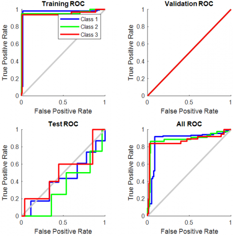
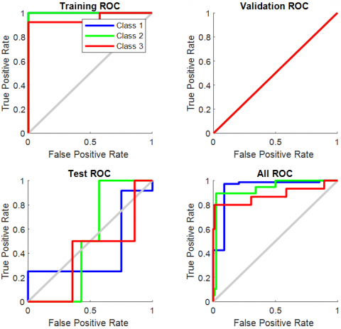
ROC curve is a schematic visualization of the potential results of a diagnostic system. It shows a trade-off between false positive and false negative rates, thereby establishing a beneficial judgment mechanism. The classification accuracy and ROC curve is used to test the output of the classifier and interpret it in context. Compared with scalar metrics such as the precision, error rate, and the error cost, the ROC graphs can provide a more rigorous estimate of the AUC (the region under the ROC curve). Figure 10 demonstrates the ROC curve produced by malignant and benign samples from the non-dense breasts collection.
Figure 10. ROC Curve of mass classification in non-dense breasts
4.4 Mass classification in dense breasts
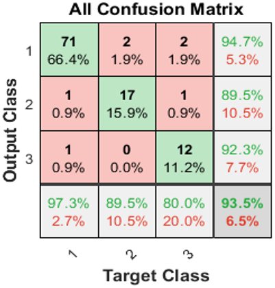
Table 9 shows three class namely Normal, benign and malign confusion matrix for dense dataset. Table 10 shows the positive and negative class calculation for each given class. Based on the TP, FP, FN and TN value, performance of the proposed mass classifier for non-dense models is calculated which is shown in Table 11.
Table 9. Confusion matrix of mass classification model for dense breasts
Table 10. Positive or negative class calculation for each given classes
|
Parameters |
Class |
Predicted class |
|
||
|
TP |
FP |
FN |
TN |
||
|
Normal image |
1 |
71 |
4 |
2 |
30 |
|
benign |
2 |
17 |
2 |
2 |
86 |
|
malign |
3 |
12 |
1 |
3 |
91 |
Table 11. Results of models applied to dense breasts dataset
|
Parameters |
Predicted class |
||
|
Normal Image |
benign |
malign |
|
|
Accuracy |
94.3 |
96.2 |
96.2 |
|
Sensitivity/Recall |
97.2 |
89.4 |
80.0 |
|
Specificity |
88.2 |
97.7 |
98.9 |
|
Precision |
94.6 |
89.4 |
92.3 |
|
F1 Score |
95.8 |
89.4 |
85.7 |
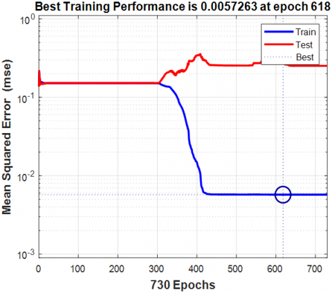
The performance graph illustrates the proposed system's performance, with respect to the number of classifications. The proposed system performance graph as seen in Figure 11. Figure 12 demonstrates the ROC curve produced by malignant and benign samples from the dense breast collection.
Figure 11. Performance graph
Figure 12. ROC Curve of mass classification in dense breasts
4.5 Comparative analysis
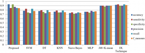
In this experiment, normal, benign and malign types of images are used as subjects. 322 distinct photographs are chosen from the dataset. In the experiment, various image features are combined to perform the experiment and the effects of which are correlated with the machine learning classification technique. Comparison of proposed method with another ML Classifier is presented in Table 7. The SVM Classifier achieved 78.24 percent accuracy and the DT and K-NN classifiers achieved 77.57 and 76.14 percent accuracy, respectively. As seen in Tables 12 the accuracy of the Naive Bayes classifier was also noticed to be above 70 percent. MLP, J48+Kmean and DL techniques achieved 76%, 90% and 92% accuracy, respectively. But our proposed method achieved the best accuracy among all techniques which is 93.24%. The values of the other output parameters such as sensitivity, accuracy, precision, recall, F-measure and gmean were prominent. The system achieved higher accuracy (0.9324), Specificity (0.9303), Precision (0.9303), Recall (0.8474) and F-measure (0.8439) against other classifiers.
Table 12. Comparative performance
|
Method |
Accuracy |
Sensitivity |
Specificity |
|
Proposed |
0.9324 |
0.8474 |
0.9303 |
|
SVM |
0.7824 |
0.8287 |
0.7439 |
|
DT |
0.7757 |
0.7960 |
0.7560 |
|
KNN |
0.7614 |
0.7890 |
0.7440 |
|
Naıve Bayes |
0.7303 |
0.7460 |
0.7140 |
|
MLP |
0.7600 |
0.7600 |
0.7400 |
|
J48+K-mean |
0.9000 |
0.9000 |
0.8800 |
|
DL Technique |
0.9200 |
0.9300 |
0.9000 |
|
Method |
Precision |
Recall |
f_measure |
|
Proposed |
0.8723 |
0.8474 |
0.8439 |
|
SVM |
0.7295 |
0.8287 |
0.7759 |
|
DT |
0.7260 |
0.7960 |
0.7536 |
|
KNN |
0.7450 |
0.7890 |
0.7494 |
|
Naıve Bayes |
0.7250 |
0.7460 |
0.7350 |
|
MLP |
0.7800 |
0.7600 |
0.7698 |
|
J48+K-mean |
0.9000 |
0.9000 |
0.9000 |
|
DL Technique |
0.9000 |
0.9300 |
0.9147 |
In this paper the combination of morphological operation and multilevel thresholding using Otsu’s technique for breast tissue segmentation compensate for the weakness of unidirectional recognition in allowing recognition rates to exceed 85 percent and more, which significantly enhances accuracy.
Figure 13 shows the comparison graph of proposed system against other machine learning algorithm on for various parameters such as accuracy, sensitivity specificity etc. From the graph we can observed that proposed method got high accuracy against all the other methods and parameters such as sensitivity, accuracy, precision, recall, F-measure and gmean are also prominent.
Figure 13. Comparison graph for skin lesion classification
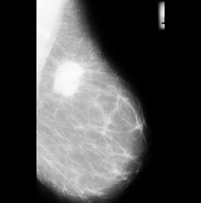
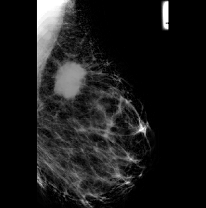
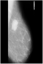
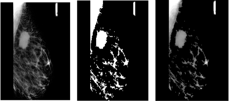
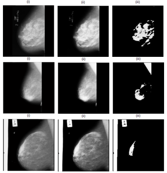
Figures 14 illustrate the outcomes of segmentation using the proposed methodology on various mammography mass pictures. The first column in each figure shows the input image, the second column the pre-processed image, and the third column the diseased region segmentation utilizing a combination of morphological operations and multi-thresholding algorithms.
Figure 14. Segmentation of images: (i) Original image, (ii) Mammography image after preprocessing step, (iii) Segmented image by combination of morphological operation and Otsu’s thresholding
An automated method for breast cancer mammography image that uses a deep learning process was first proposed. The noise handling and resizing techniques are used to define the pre-processing phase, which is crucial. We used a multi-level thresholding technique for cancer area segmentation. Different colour and texture features are retrieved and input into the network for classification, which is done using DNN. In our work, we've constructed three DNN models. First, we construct a model to categorise breast tissue as dense or non-dense, and then we create two models based on dense breasts to identify parts of the breast as mass or non-mass. The proposed DL technique outperformed state-of-the-art techniques, according to the quantitative analysis and validation.
The limitation of this proposed approach is that it requires a large amount of time. Since we are using three types of deep learning models, so it takes more time to run on small size datasets. The transfer learning approach can be used to increase the efficiency of the system.
The goal in the future is to build a large-scale network of deep learning with transfer learning approach to assist radiologists in accurately validating massive datasets in less time.
[1] Rathi, M., Pareek, V. (2016). Hybrid approach to predict breast cancer using machine learning techniques. International Journal of Computer Science Engineering, 5(3): 125-136.
[2] Tahmooresi, M., Afshar, A., Rad, B.B., Nowshath, K.B., Bamiah, M.A. (2018). Early detection of breast cancer using machine learning techniques. Journal of Telecommunication, Electronic and Computer Engineering (JTEC), 10(3-2): 21-27.
[3] Aslan, M.F., Celik, Y., Sabancı, K., Durdu, A. (2018). Breast cancer diagnosis by different machine learning methods using blood analysis data. International Journal of Intelligent Systems and Applications in Engineering, 6(4): 289-293. https://doi.org/10.18201/ijisae.2018648455
[4] Shravya, C., Pravalika, K., Subhani, S. (2019). Prediction of breast cancer using supervised machine learning techniques. International Journal of Innovative Technology and Exploring Engineering, 8(6): 1106-1110.
[5] Wadkar, K., Pathak, P., Wagh, N. (2019). Breast cancer detection using ANN network and performance analysis with SVM. International Journal of Computer Engineering and Technology, 10(3): 75-86.
[6] Dheeba, J., Singh, N.A., Selvi, S.T. (2014). Computer-aided detection of breast cancer on mammograms: A swarm intelligence optimized wavelet neural network approach. Journal of Biomedical Informatics, 49: 45-52. https://doi.org/10.1016/j.jbi.2014.01.010
[7] Subashini, K., Jeyanthi, K. (2014). Masses detection and classification in ultrasound images. IOSR Journal of Pharmacy and Biological Sciences, 9(3): 48-51.
[8] Antony, S.J.S., Ravi, S. (2014). Breast cancer detection on thermogram at preliminary stage by using fuzzy inferences system. Journal of Theoretical and Applied Information Technology, 68(3): 381-391.
[9] Radovic, M., Djokovic, M., Peulic, A., Filipovic, N. (2013, November). Application of data mining algorithms for mammogram classification. In 13th IEEE International Conference on BioInformatics and BioEngineering, Chania, Greece, pp. 1-4. https://doi.org/10.1109/BIBE.2013.6701551
[10] de Oliveira Martins, L., Silva, A.C., De Paiva, A.C., Gattass, M. (2009). Detection of breast masses in mammogram images using growing neural gas algorithm and Ripley’s K function. Journal of Signal Processing Systems, 55(1): 77-90. https://doi.org/10.1007/s11265-008-0209-3
[11] Anjaiah, P., Prasad, K.R., Raghavendra, C. (2018). Effective texture features for segmented mammogram images. International Journal of Engineering & Technology, 7(3): 666-669. https://doi.org/10.14419/ijet.v7i3.12.16450
[12] Fonseca, P., Mendoza, J., Wainer, J., Ferrer, J., Pinto, J., Guerrero, J., Castaneda, B. (2015). Automatic breast density classification using a convolutional neural network architecture search procedure. Medical Imaging 2015: Computer-Aided Diagnosis, 9414: 556-563. https://doi.org/10.1117/12.2081576
[13] Ahn, C.K., Heo, C., Jin, H., Kim, J.H. (2017). A novel deep learning-based approach to high accuracy breast density estimation in digital mammography. Medical Imaging 2017: Computer-Aided Diagnosis, 10134: 691-697. https://doi.org/10.1117/12.2254264
[14] Li, S., Wei, J., Chan, H.P., et al. (2018). Computer-aided assessment of breast density: comparison of supervised deep learning and feature-based statistical learning. Physics in Medicine & Biology, 63(2): 025005. https://doi.org/10.1088/1361-6560/aa9f87
[15] Kyono, T., Gilbert, F.J., van der Schaar, M. (2018). MAMMO: A deep learning solution for facilitating radiologist-machine collaboration in breast cancer diagnosis. arXiv preprint arXiv:1811.02661.
[16] Zhang, X., Zhang, Y., Han, E.Y., Jacobs, N., Han, Q., Wang, X., Liu, J. (2018). Classification of whole mammogram and tomosynthesis images using deep convolutional neural networks. IEEE Transactions on Nanobioscience, 17(3): 237-242. https://doi.org/10.1109/TNB.2018.2845103
[17] Shen, L., Margolies, L.R., Rothstein, J.H., Fluder, E., McBride, R., Sieh, W. (2019). Deep learning to improve breast cancer detection on screening mammography. Scientific Reports, 9(1): 12495. https://doi.org/10.1038/s41598-019-48995-4
[18] Tardy, M., Scheffer, B., Mateus, D. (2019). Breast density quantification using weakly annotated dataset. In 2019 IEEE 16th International Symposium on Biomedical Imaging (ISBI 2019), Venice, Italy, pp. 1087-1091. https://doi.org/10.1109/ISBI.2019.8759283
[19] Shen, T., Gou, C., Wang, J., Wang, F.Y. (2019). Simultaneous segmentation and classification of mass region from mammograms using a mixed-supervision guided deep model. IEEE Signal Processing Letters, 27: 196-200. https://doi.org/10.1109/LSP.2019.2963151
[20] Wang, Y., Lei, B., Elazab, A., et al. (2020). Breast cancer image classification via multi-network features and dual-network orthogonal low-rank learning. IEEE Access, 8: 27779-27792. https://doi.org/10.1109/ACCESS.2020.2964276
[21] Song, R., Li, T., Wang, Y. (2020). Mammographic classification based on XGBoost and DCNN with multi features. IEEE Access, 8: 75011-75021. https://doi.org/10.1109/ACCESS.2020.2986546
[22] Ribli, D., Horváth, A., Unger, Z., Pollner, P., Csabai, I. (2018). Detecting and classifying lesions in mammograms with deep learning. Scientific Reports, 8(1): 4165. https://doi.org/10.1038/s41598-018-22437-z
[23] Jung, H., Kim, B., Lee, I., et al. (2018). Detection of masses in mammograms using a one-stage object detector based on a deep convolutional neural network. PloS One, 13(9): e0203355. https://doi.org/10.1371/journal.pone.0203355
[24] Lin, T.Y., Goyal, P., Girshick, R., He, K., Dollár, P. (2017). Focal loss for dense object detection. In Proceedings of the IEEE International Conference on Computer Vision, Venice, Italy, pp. 2980-2988. https://doi.org/10.1109/ICCV.2017.324
[25] Morrell, S., Wojna, Z., Khoo, C.S., Ourselin, S., Iglesias, J.E. (2018). Large-scale mammography cad with deformable conv-nets. In: , et al. Image Analysis for Moving Organ, Breast, and Thoracic Images. RAMBO BIA TIA 2018 2018 2018. Lecture Notes in Computer Science(), vol 11040. Springer, Cham. https://doi.org/10.1007/978-3-030-00946-5_7
[26] Morrell, S., Wojna, Z., Khoo, C.S., Ourselin, S., Iglesias, J.E. (2018). Large-scale mammography CAD with deformable conv-nets. In Image Analysis for Moving Organ, Breast, and Thoracic Images, Granada, Spain, pp. 64-72. https://doi.org/10.1007/978-3-030-00946-5_7
[27] Halling-Brown, M.D., Looney, P.T., Patel, M.N., Warren, L.M., Mackenzie, A., Young, K.C. (2014). The oncology medical image database (OMI-DB). In Medical Imaging 2014: PACS and Imaging Informatics: Next Generation and Innovations, 9039: 25-31. https://doi.org/10.1117/12.2041674
[28] Dream challenge: The digital mammography Dream challenge (2017). https://www.synapse.org/#!Synapse:syn4224222/wiki/401743.
[29] Agarwal, R., Díaz, O., Yap, M.H., Lladó, X., Martí, R. (2020). Deep learning for mass detection in full field digital mammograms. Computers in Biology and Medicine, 121: 103774. https://doi.org/10.1016/j.compbiomed.2020.103774
[30] https://www.kaggle.com/kmader/mias-mammography, accessed on 25 Nov. 2021.
[31] Rajpoot, V., Dubey, R., Khan, S.S., Maheshwari, S., Dixit, A., Deo, A., Doohan, N.V. (2022). Orchard Boumans algorithm and MRF approach based on full threshold segmentation for dental X-ray images. Traitement du Signal, 39(2): 737-744. https://doi.org/10.18280/ts.390239
[32] Trivedi, V.K., Shukla, P.K., Pandey, A. (2022). Automatic segmentation of plant leaves disease using min-max hue histogram and k-mean clustering. Multimedia Tools and Applications, 81: 20201-20228. https://doi.org/10.1007/s11042-022-12518-7