Kanchana Rajendran* | Menaka Radhakrishnan | Sethuraman Viswanathan
© 2022 IIETA. This article is published by IIETA and is licensed under the CC BY 4.0 license (http://creativecommons.org/licenses/by/4.0/).
OPEN ACCESS
The human brain is the body's most complicated organ. Constant blood flow is essential for the sustained functioning of the brain. A blocked blood vessel's interruption of blood supply prevents oxygen and nutrients to the brain tissues. This results in a life-threatening brain disease called Ischemic Stroke. Computed Tomography (CT) images are widely used in the diagnosis of Ischemic Stroke because of their faster acquisition and compatibility with most life support devices. CT acquired from the patients who arrived with stroke symptoms is Primary CT (PCT). After some hours CT taken for the same patient is Secondary CT (SCT). Stroke lesions may not be visible in PCT, whereas visible in SCT. Learning the features automatically using a Convolutional Neural Network (CNN) is essential to classify normal and abnormal CT slices. These networks are capable of learning the global features effectively for image classification. Though this CNN approach works, achieving desired accuracy was challenging. Different architectures considered for this CNN experimentation are VGG1, VGG2, VGG3, VGG16, InceptionV3, and ResNet50. This novel work provides a detailed explanation of the three experiments conducted using PCT and SCT slices. Three experiments are conducted using SCT and PCT slices. The pretrained VGG16, ResNet50, and InceptionV3 networks with the ImageNet database are applied as a first approach. Both SCT and PCT slices are used for testing alone. It resulted in 49.22%, 47.076% and 49.36% classification accuracy. In the second approach, different models were trained for classification from PCT and SCT slices. This includes the networks like VGG1, VGG2, VGG3, VGG16, VGG16 with dropout, ResNet, ResNet50 with lambda regularization, InceptionV3, and InceptionV3 with lambda regularization. The accuracies achieved are 68%, 69.4%, 72%, 78.2%, 79.1%, 77%, 77.8%, 79.6% and 80.1%. The accuracy was improved with dropout and lambda regularization. The networks with high accuracy are selected and an ensemble model is developed as a third approach. ResNet50, VGG16, and InceptionV3 are combined to form an ensemble network. This ensemble network yielded an accuracy of 81.98% when SCT and PCT slices are used for both training and testing. And produced 74% accuracy when PCT slices alone were used. Also produced 93.76% accuracy when SCT slices alone were used.
Ischemic Stroke, CT, CNN, VGG16, InceptionV3, Resnet50, ensemble network
Stroke is the leading cause of death and disability in the developing world, impacting one in every six people and resulting in an estimated three to six million Stroke cases per year. The most significant and dangerous cerebrovascular condition is a Cerebral Vascular Accident (CVA), which is one of the leading causes of global death, next to heart attack [1]. Stroke survivors are more likely to have sudden problems, with Stroke being the leading cause of adult epilepsy. It can be classified as either an Ischemic (blockage of insufficient blood flow) or a Hemorrhagic (bleeding) Stroke (blood vessel break). Ischemic Stroke accounts for 80-85% of all Strokes. A thrombotic or embolic blockage of a cerebral artery causes an acute Ischemic Stroke. Deep ischemia is caused by occlusion of the proximal cerebral artery, which results in a collapse of cellular energetics. In a few minutes, necrotic cell death occurs. A partial area of Ischemia, called the penumbra, surrounds the infarct core, where neurons will die within hours. Patients who would benefit the most from treatment could be identified by accurately identifying this "tissue at risk". The extent of damage in a massive Ischemic Stroke will worsen during the next few days. In the worst-case scenario, the mass effect combined with tissue injury causes a rise in intracranial pressure and a loss of cerebral blood flow.
Recently, Stroke detection using devices such as Computed Tomography (CT) and Magnetic Resonance Imaging (MRI) has enabled a skilled radiologist to determine whether or not a patient has suffered a Stroke. On non-Contrast Computed Tomography (NCCT) scans, measuring the volume of infarcts gives a quantitative assessment of infarcted brain tissue caused by an Ischemic Stroke. The volume of a follow-up infarct measured 24 hours after onset is a good predictor of functional prognosis. Multiple randomized controlled trials have proposed infarct volume as a surrogate goal for traditional patient outcome scales. A more exact prediction of the patient outcome can be produced by integrating infarct volume and infarct location. A manual delineation by medical experts is the gold standard for infarct segmentation. Manual demarcation, on the other hand, has various drawbacks, including the fact that it is time-consuming, subjective, prone to errors, and costly. For image classification and segmentation, Convolutional Neural Networks (CNNs) have outperformed several existing image analysis approaches. CNNs have performed well in a variety of medical imaging areas, including the segmentation of ischemic stroke lesions in brain CT images. The utility of CNNs for automatic segmentation of infarcted brain tissue in follow-up NCCT scans from patients with an acute ischemic stroke was investigated in this work.
When a patient reaches the hospital with ischemic lesion symptoms, the initially recommended modality is CT. This is termed Primary CT (PCT). Based on the observation in PCT, the doctor will decide whether it is an Ischemic lesion or a hemorrhagic lesion. In most cases, even if the lesion region is present, it will not be visible in the scanned image slices. After four hours, a Secondary CT (SCT) is recommended and within this period stroke lesion becomes visible in the slice. The period between the PCT and SCT is very crucial.
Any delay makes the patient’s life at risk. Though the PCT looks normal for a human eye, intensity variations will be present in the stroke lesion region. By advancing image processing algorithms if this intensity variation could be captured in PCT, it will help the medical fraternity on a larger scale. Classifying the PCT image slices and segmenting the IS lesion from PCT becomes essential for analysis. This research work focuses on the classification of PCT and SCT slices.
Three-dimensional CNN system was proposed to identify Ischemic Stroke from CT angiography source images (CTA-SI) [2]. Stroke symptoms can be diagnosed in a short period using deep learning algorithms [3].
A multi-scale CNN (U-Net) and a convolutional auto- encoder are utilized to forecast ischemic stroke lesion tissues [4, 5]. 10-point CT-scan score can be used to identify patients with acute Ischemic Stroke [6]. The purpose of this study is to develop an automated Alberta Stroke Programme Early CT Score (ASPECTS) scoring system that analyses CT images using binary classification and a three-dimensional CNN to enhance decision-making.
CT scans are used to demonstrate a CNN method for automatically classifying strokes [7]. CT Perfusion (CTP) is employed to triage early-stage Ischemic Stroke patients [8]. An automated early Ischemic Stroke detection method is developed using a CNN deep learning algorithm [9, 10]. After obtaining the CT slices of the brain, the system will do picture pre-processing to eliminate the improbable area that is not the likely Stroke area. Deep learning system is proposed for learning and categorization Ischemic Stroke [11].
An excellent pre-processing technique for Ischemic Stroke is performed using non-contrast CT data from the Middle Cerebral Artery (MCA) region. Furthermore, the adaptive transfer learning method was proposed in this study, which improves the transfer learning module to address the problem of limited data when training neural networks. When it comes to diagnosing Strokes, the proposed method outperformed the current system by 18.72 percent. Artificial Intelligence (AI) can help in infarct or hemorrhage detection, segmentation, classification, major vascular occlusion detection, ASPECTS grading, and prognostication, among other aspects of the Stroke therapy paradigm [12, 13].
The purpose of this research is to introduce AI methodologies and existing public and commercial platforms in Stroke imaging, as well as to summarize the literature on current AI-driven applications for acute Stroke triage, surveillance, and prediction. The use of CT imaging for patients with stroke symptoms is a crucial step in the triaging and diagnostic process [14, 15]. It is described how to use an automated deep learning algorithm to segment acute stroke lesion cores from CT and CT perfusion images. This method is compared to other cutting-edge methods using a blind testing set evaluation on the challenge website, which maintains a current leaderboard for fair and direct method comparisons.
A tool is proposed that earns a competitive performance rating among the top- performing methods on the Ischemic Stroke Lesion Segmentation Challenge 2018 (ISLES18) testing leaderboard, with an average Dice similarity coefficient of 49% [16, 17]. Without the need for time-consuming MRI, this approach can provide a clinical assessment of lesion core size and location. As a public resource, the described technology is made available to the scientific community. The appearance of the contralateral anatomy, as well as the atlas-encoded spatial location, are combined using CNN architecture. Contextual information’s are used to identify Stroke signs [18, 19]. Using widely available NCCT and CT angiography (CTA) data, deep learning can be employed to identify lesions [20].
A multi-scale 3D CNN with NCCT, CTA, and CTA (8 s delay after CTA) images as inputs was used to create the predictive model. CNN model is developed using image fusion and CNN algorithms [21]. The CT image dataset is partitioned into 20% testing and 80% training sets in the first experiment, and the image dataset is cross-validated 10 times in the second trial.
CT imaging is employed to diagnose ischemia in the Posterior Fossa (PF), which is a conventional method for diagnosing Ischemia [22]. Machine learning's practical performance is being put to the test with the advent of deep learning applications in healthcare. This is the first study to look at the use of deep transfer learning in brain CT images in the posterior area for automated Ischemia classification. The testing results demonstrate that ResNet50 is capable of reaching the maximum accuracy performance when compared to other proposed models. Overall, this automated classification is a useful and time-saving technique for improving medical diagnosis.
Random forest algorithm is used to substitute Neural Network (NN) in CNN to provide an update in the identification of Ischemic Stroke based on patient CT scans [23]. As a result, while classifying data, the fully connected layer on CNN is completely replaced by random forests following feature extraction. CNN optimized via Particle Swarm Optimization is a novel research technique [24]. This is done to overcome the problem of stroke detection in CT scans.
Significant need to swiftly and correctly analyze aging data can be done in Stroke because of the multiple potential AI applications [25]. AI could be beneficial to neuroradiologists. More standardized imaging data sets and more detailed AI experiments are needed to establish and validate the usefulness of AI in stroke imaging. Deep learning algorithms have a significant impact on stroke diagnosis, treatment, and prediction [26, 27]. This study also discusses the current limitations and future development prospects of deep learning technology.
Deep learning models with fine-tuning outperform standard thresholding methods in terms of predicting tissue at risk and ischemic core.
Developing a computer-aided automated method to aid in locating acute lesions is necessary. A broad review on stroke along with detection modalities and methods to develop a computer-aided approach to detect acute lesions. A computer- aided diagnosis system is to be developed to help radiologists to diagnose brain stroke for treatment plans at a much faster pace.
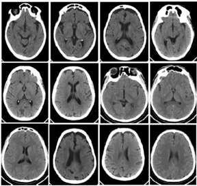
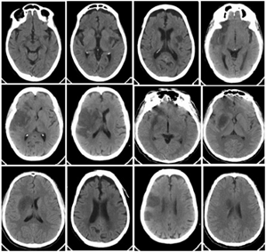
PCT and SCT Ischemic Stroke datasets were collected from Global Health City, Chennai, and Sri Ramachandra Institute of Higher Education and Research, Chennai. The collected datasets were in the video stream. Those video streams are then converted into image sequences using video to image converter software. A total of 1120 Normal CT (NCT) slices, 2400 SCT slices and 960 PCT slices were obtained and used for this research work. The lesion regions were manually marked by the radiologists. This is used as ground truth. Sample PCT slices are shown in Figure 1. Also, Figure 2 shows sample SCT slices.
Figure 1. PCT slices
Figure 2. Corresponding SCT slices
Data augmentation is required to increase the sample size. It is done in the ratio of 1:2. 2400 SCT, 960 PCT slices and 1120 NCT slices are subjected to augmentation. Hence, 4800 SCT, 1920 PCT and 2240 NCT slices are generated as a result of data augmentation. When the model is exposed to a high number of data samples, the risks of overfitting the training data are greatly reduced. Zoom factor (12%), shearing (10%), rotation (30 degrees), horizontal flipping (40%), vertical flipping (40%) and shifting (15%), are the geometric transformations applied for augmenting the dataset. Machine learning algorithms need a sample dataset to train the model when they are created. The model, however, may begin to learn the irrelevant information within the dataset if it trains on sample data for an excessively long time or if the model is overly complex. The model becomes "overfitted" and unable to generalize successfully. A model won't be able to carry out the classification or prediction tasks that it was designed for if it can't generalize successfully to new data. To overcome such issues, dropout, regularization techniques and ensemble learning methods are used. The most popular ensemble techniques are boosting and bagging. Following the generation of several data samples, these models are individually trained, and depending on the task like, classification or regression, the average or majority of those predictions result in a more accurate estimate. This is frequently employed to lower variance in a noisy dataset.
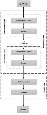
Figure 3. Basic convolutional neural network
CNN can be considered as one of the special cases of Feed-Forward Neural Networks (FNN). The neurons of each layer in the conventional neural network are one-dimensional. But in CNN, these layers have three dimensions namely height, width, and depth. Basic CNN architecture in Figure 3 shows a convolutional layer, pooling layer, and fully connected layer. Feature learning is done in the convolution blocks and classification is done in the fully connected and softmax layer.
Convolution is the concept of sliding a filter over the input. It represents an understanding of features within an image. To extract these features filters are used. Several filters in the network are kernels. It is a process of transforming an image by applying a kernel over each pixel. Downsampling is done by a pooling layer to reduce the size of the feature maps. The pooling layers apply the max of mean, max-pooling or average pooling to downsample the feature map. To preserve the edges of the images, zero is padded to the edges of the images. A fully connected layer predicts the image class using the information obtained in earlier epochs. This will enable the machine to learn from the extracted features and create a generalized model. The network architecture was built by removing the final classification layer and the transfer learned for our CT classification.
Several experiments have been carried out to increase the network's performance by adjusting the parameters used. The method followed for hyper parameter adjustment was grid search. Grid search is a process that searches exhaustively through a manually specified subset of the hyper parameter space of the targeted algorithm. This helped us arrive in an optimum subspace of hyper parameters. To classify the normal and abnormal CT slices, three experiments are carried out. CNN-based deep learning networks are used to perform the classification. Experiments 1 and 2 are conducted with pretrained architectures. In experiment 1 transfer learning is applied. In experiment 2, the pretrained networks are trained with PCT and SCT slices. In experiment 3, ensemble architecture is developed and the accuracy is improved.
The pre-trained networks VGG16, ResNet50, and InceptionV3 are chosen for the first experiment. These networks are trained with the ImageNet dataset and the weights are frozen. The ImageNet is a vast visual database created for visual object recognition that comprises over fourteen million images organized into 20,000 categories, of generic images. The knowledge gained from the source dataset (generic images) is transferred to the target dataset (PCT and SCT slices) using transfer learning. Through the transfer learning approach, the knowledge gained by the ImageNet dataset is leveraged to classify the slices with the lesion. Except for the output layer, the target model duplicates and fine-tunes all of the source model parameters using the target dataset. The target model’s output layer, on the other hand, is trained from scratch. When fine-tuning parameters, a lower learning rate is employed, but when training the output layer from scratch, a higher learning rate is used. A learning rate of 0.001, and a weight decay factor of 0.01 with a momentum value of 0.9 is applied. The initial layers of all the CNN models are pretrained on the ImageNet dataset and only the final layer is fine-tuned for the purpose of this domain shift. The SCT and PCT slices are submitted to the pretrained networks for classification as normal or abnormal. The initial layers of the model are learning the features from the ImageNet dataset and learning carried out only by the final layer is not sufficient to perform the classification. To overcome this challenge all the initial layers of the model are unfrozen and training is carried out with PCT and SCT slices from scratch. A rise in accuracy is observed as soon as the domain shift is addressed. The classification accuracy produced by VGG16, ResNet50, and InceptionV3 is 49.22%, 47.076%, and 49.36%. The average accuracy is observed to be around 48% which is due to the domain shift in the training and testing images.
In this experiment, VGG1, VGG2, VGG3, VGG16, ResNet50, InceptionV3 architectures are trained with PCT and SCT slices. To improve accuracy dropout regularization and lambda regularization are applied for VGG16, ResNet50 and InceptionV3.
8.1 VGG architecture
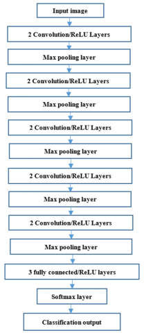
VGG stands for Visual Geometry Group and is a multilayer deep CNN architecture. The term "deep" refers to the number of layers in VGG. VGG1, VGG2, VGG3, and VGG16 are 1, 2, 3, and 16-layer convolutional layers, respectively. VGG architecture is the foundation for cutting-edge object recognition models [28]. The input CT image is resized to the size of the networks. Instead of a convolution layer with a large kernel size, VGG groups multiple convolution layers with smaller kernel sizes. More layers in VGG allowed the model to better understand the features within an image. The convolutional layers are generally composed of 3×3 filters. The Maximum Pooling (Max-Pool) layer follows the convolution layer, not necessarily all convolution layer has a max-pool layer. A stack of convolutional layers with a narrow receptive field is used to process the image. In CNN, the Rectified Linear Unit (ReLU) is one of the most commonly utilized activation functions. If the input value is less than zero, the output of a rectified linear unit is '0'. Otherwise, it displays the raw input as the output, i.e., if the input value is larger than zero, it suggests that the output is equal to the input value. All hidden layers are equipped with the ReLU activation function. A learning rate of 0.001, and a weight decay factor of 0.01 with a momentum value of 0.9 is applied. The network is converged in 40 epochs. Figure 4 shows the VGG16 architecture.
Classification Accuracy (CA) is calculated using the number of correct predictions and the total number of predictions made. This value is multiplied by 100 to present it in percentage. An optimization function's goal is to maximize or minimize an error function, which is determined by the model's internal learning parameters such as bias and network weights.
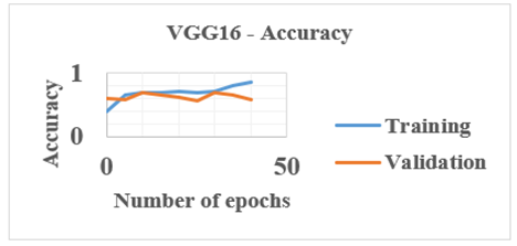
Adaptive Moment Estimation (Adam) optimization is one of the optimization functions investigated in this study. A loss function determines the "quality" of a neural network's performance in terms of classification output. For training the network, cross-entropy is the loss function used. The difference between two probability distributions is measured by cross-entropy. The target distribution will look closer to the actual distribution if the cross-entropy values are minimized. To figure out the classification accuracy and cross-entropy loss, the PCT and SCT slices are employed for training, testing, and validation. This VGG1, VGG2, VGG3, and VGG16 produced a CA of 68%, 69.4%, 72%, and 78.2%. Figure 5 shows the results of VGG16.
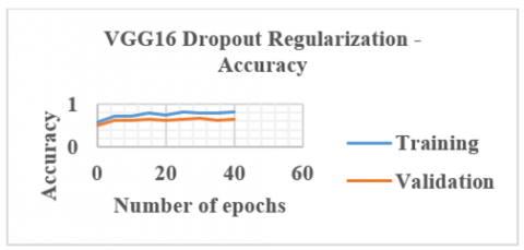
The dropout technique is applied to the VGG16 network to improve classification accuracy. It is a training method in which neurons are rejected at random. They mysteriously "vanish." This means that their contribution to the activation of downstream neurons is removed temporally on the forward pass, and no weight updates are applied to the cell on the backward trip. Likelihood of dropping out for each layer introduced in a dense network. Each neuron has a chance of getting skipped over throughout each iteration. Overfitting is a type of modeling error that arises when a function is too closely related to a certain set of data. This regularization technique prevents complex co-adaptations on training data, hence reduces overfitting. VGG16 network is applied with dropout regularization and this produced an improved of 79.1%. The output obtained by applying the dropout technique is presented in Figure 6.
Figure 4. VGG16 architecture
Figure 5. VGG16 accuracy plot
Figure 6. VGG16 with dropout regularization accuracy plot
8.2 ResNet50
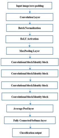
Figure 7. ResNet50 architecture
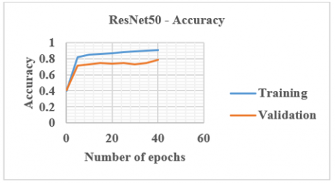
Residual Neural Network (ResNet) was introduced in 2015. It also addressed the problem of disappearing gradients in very deep neural networks. It is a variant of ResNet with 48 Convolution layers, 1 MaxPool layer, and 1 Average Pool layer. ResNet50 is a deep neural network that may be used for a range of computer vision tasks like object detection and image segmentation. Residual nets with up to 152 layers of depth - 8 times deeper than VGG nets but with lower complexity. Each 2-layer block in the 34-layer net is replaced with a 3-layer bottleneck block resulting in a 50-layer ResNet. Instead of using a complicated adaptive learning technique, plain Stochastic Gradient Descent (SGD) is used. This is done in conjunction with an acceptable initialization function that preserves the training modifications in preprocessing the input, which divides the input into patches before feeding it into the network. In this network, no need to fire all neurons for every epoch. Once learnt, not trying to learn again, instead focuses on learning newer features. This greatly reduces the training time and improves accuracy. The degradation problem raised by the VGG network is solved by residual learning. Figure 7 shows the ResNet50 architecture. Figure 8 shows the accuracy plot of ResNet50.
Figure 8. ResNet50 accuracy plot
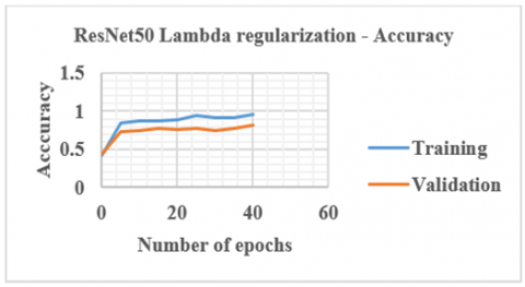
Figure 9. ResNet50 with Lambda regularization accuracy plot
Once training is carried out using the PCT and SCT slices, a CA of 77% is achieved. Lambda regularization is a strategy for improving model generalization by making minor changes to the learning procedure. As a result, the model's performance on previously unseen data improves as well. Using the regularizers, we may apply regularization to any layer directly. To improve accuracy, lambda regularization is applied and this resulted in 77.8% CA. Figure 9 presents the responses obtained using ResNet50 with lambda regularization.
8.3 InceptionV3
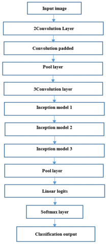
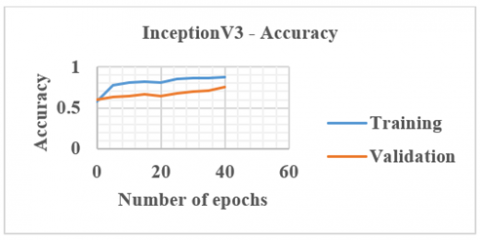
InceptionV3 is a CNN design from the Inception family that transports label information down the network using label smoothing, factorized 7 x 7 convolutions, and an auxiliary classifier. Batch normalization is used frequently throughout the model and is applied to activation inputs. In addition to digging deeper, the researchers devised a revolutionary technique called the Inception module [29]. Multiple feature extraction, adaptable filter size and extracting features at varied scales are the advantage of InceptionV3. This network avoids representational bottlenecks. It means it reduces the input dimensions of the next layer. It has multiple deep layers of convolutions which may result in overfitting. To avoid it, multiple filters of different sizes are used. Hence this architecture uses parallel layers, instead of deep layers, thus making the network wider. Figure 10 shows the InceptionV3 architecture. The size of various layers is shown in Table 1. Figure 11 presents the networks outputs.
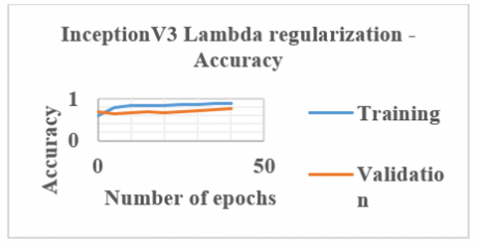
Once training, testing and validation are carried out using the PCT and SCT slices, CA is calculated as 79.6%. Also, after applying the lambda regularization technique to this InceptionV3 network, CA is improved to 80.1%. Figure 12 shows the output obtained using the InceptionV3 network with lambda regularization.
Figure 10. InceptionV3 architecture
Figure 11. InceptionV3 accuracy plot
Table 1. Various layer sizes of InceptionV3 architecture
|
S. No |
Type |
Patch size/stride |
|
1 |
Convolution layer |
3×3/2 |
|
2 |
Convolution layer |
3×3/1 |
|
3 |
Convolution padded |
3×3/1 |
|
4 |
Pooling layer |
3×3/2 |
|
5 |
Convolution layer |
3×3/1 |
|
6 |
Convolution layer |
3×3/2 |
|
7 |
Convolution layer |
3×3/1 |
|
8 |
Inception model1 |
Module1 |
|
9 |
Inception model2 |
Module2 |
|
10 |
Inception model3 |
Module3 |
|
11 |
Pooling layer |
8×8 |
|
12 |
Linear |
logits |
|
13 |
Softmax |
classifier |
Once training, testing and validation are carried out using the PCT and SCT slices, CA is calculated as 79.6%. Also, after applying the lambda regularization technique to this InceptionV3 network, CA is improved to 80.1%. Figure 12 shows the output obtained using the InceptionV3 network with lambda regularization.
Figure 12. InceptionV3 with lambda regularization accuracy plot
Precision is about what percentage of all the optimistic predictions is genuinely positive. Its value ranges from 0 to 1. The recall is about what proportion of the total positive is anticipated to be positive. The harmonic mean of precision and recall is the F1 score. It considers both false positives and false negatives. As a result, it works well with an unbalanced dataset. The parameters recall, precision and the F1 score obtained for the models are presented in Table 2.
Table 2. Parameters of the models
|
S.No |
Models |
Recall |
Precision |
F1 score |
|
1 |
VGG1 |
0.51 |
0.53 |
0.51980769 |
|
2 |
VGG2 |
0.57 |
0.55 |
0.55982143 |
|
3 |
VGG3 |
0.58 |
0.6 |
0.58983051 |
|
4 |
ResNet50 |
0.61 |
0.6 |
0.60495868 |
|
5 |
VGG16 |
0.65 |
0.61 |
0.62936508 |
|
6 |
InceptionV3 |
0.67 |
0.61 |
0.63859375 |
A neural network ensemble is a learning paradigm that solves a problem by combining multiple neural networks. Ensemble learning combines predictions from many neural network models to reduce prediction variation and generalization errors [30]. It is a machine-learning technique that mixes numerous base models to create a single best-predictive model. This is done because ensembles perform better in terms of generalization than a single network. Each model is allowed to generate a prediction and the final prediction being the average of the individual prediction.
The convolution layer, rectified unit layer, pooling layer, and connected layer are the CNNs basic layers. The pixels are grouped in a CNN technique, which is subsequently processed by filters. Depending on the complexity of the training data, the number of filters can be adjusted. The pooling layer then does regression or reduces the input parameters. This process is repeated over and over on the same data in an ensemble approach to produce a more dependable decision.
The traditional hyper parameters of the network was kept the same but final layer was altered using the learning rate of 0.001, and a weight decay factor of 0.01 with a momentum value of 0.9.
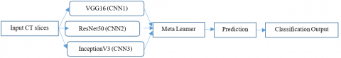
Here in this research, the trained models with the highest accuracy as VGG16 with dropout regularization, ResNet50 and InceptionV3 with lambda regularization, are concatenated to form an Ensemble architecture which is shown in Figure 13.
A concatenation ensemble takes many inputs of varying dimensions and concatenates them on a single axis. Concatenation operations are the polar opposite of averaging ensemble activities. The average is computed by passing the pooled outputs of the networks through dense layers with a set number of neurons to equalize them. Weighted ensembles are a type of averaging operation in which the tensor outputs are multiplied by a weight and then blended linearly.
For sampling data from the training set, there are two main approaches.
1. Bootstrap AGGregating, or BAGGing: It is called BAGGing because it combines Bootstrapping and Aggregation into a single ensemble model. It takes replacement samples from the training set at random. It separates the original training set into multiple training sets, each of which is used to train a component neural network separately. For every single data sample, several bootstrapped subsamples are generated.
2. Boosting: This approach trains machine learning models sequentially, rather than concurrently, as in traditional ensemble methods. Adaptive boosting (AdaBoost) is the boosting algorithm that is used for classification and regression [31].
When a machine learning model performs well on training data but not so well on real-world samples, this is known as overfitting. Ensemble learning can be used to overcome this problem. Machine learning ensembles are made up of several decision trees known as random forests [32].
Explainability is an issue with ensemble learning. It is simple to trace a single machine learning model, such as a decision tree. Understanding the rationale behind each decision gets significantly more difficult when hundreds of models contribute to an outcome.
Since VGG16 with dropout regularization, ResNet50 with lambda regularization and InceptionV3 with lambda regularization produced CA of 79.1%, 77.8%, and 80.1%, these networks are selected to make ensemble architecture. This architecture is designed in such a way that VGG16, ResNet50, and InceptionV3 are connected to the decision-making model. This decision-making model is a voting mechanism.
Following are the steps followed in the ensemble CNN model for classification.
Figure 13. Proposed Ensemble CNN model
1. The objective behind the Ensemble model is to classify the PCT slices. An Ensemble network is a collection of CNN, each classifies according to the input. The input slices given to the ensemble networks are given in Eq. (1).
Input CT slice =[PCT, SCT, NCT] (1)
Each network produces the membership probabilities (pb1, pb2,….., pbn), where pb1+pb2+……+pbn=1 and n is the number of networks used. Each CNNs probability is joined and given to the meta learner. This meta learner with its voting mechanism decides to generate the output.
2. In the proposed ensemble, VGG16, ResNet50 and InceptionV3 are the considered CNN’s given in Eq. (2). All these networks do their work in parallel mode and give the result.
Networks used= [VGG16, ResNet50, InceptionV3] (2)
3. Each of these CNN has a number of convolutional blocks with a convolution layer and pooling layer. A various number of filters with variable sizes are used in the convolution layer. Once the convolution operation is over, ReLU function is applied to it. At last dropout rate is included as an optional factor taking values from 0 to 1. A fully connected layer with a variable number of units is included which is ended with a softmax function. From this last unit, the final membership probability is computed.
4. Three cases are considered for training, testing and validation using SCT, PCT and NCT. Those three dataset combinations are given in Eq. (3).
Dataset combinations = [(PCT and NCT), (PCT, SCT, and NCT), (SCT and NCT)] (3)
5. Networks in the Ensemble CNN uses this dataset combination and produces its output to the meta learner. Tunable parameters are fine-tuned to attain the maximum classification accuracy, thereby reducing the errors. 4800 SCT, 1920 PCT and 2240 NCT slices are the datasets used in this work. The training phase is done using the 80% and validation using the 20% dataset. Once training is over, the network is tested and validated in the way given in Eq. (4).
Dataset=[80% training, 20% validation] (4)
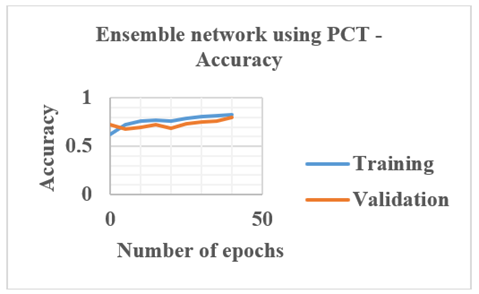
6. When PCT and NCT datasets are used, 1536 PCT and 1792 NCT slices are meant for training. 384 PCT and 448 NCT slices are meant for validation. Ensemble network using these datasets is given in Eq. (5). Figure 14 shows the ensemble networks accuracy plot when PCT slices are used.
[Ensemble Architecture](PCT,NCT)=[Training, Testing and Validation](PCT,NCT) (5)
Figure 14. Accuracy plot of Ensemble network using PCT
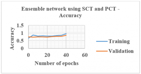
7. When PCT, SCT and NCT datasets are used, 1536 PCT, 3840 SCT and 1792 NCT slices are meant for training. For validation, 384 PCT, 960 SCT and 448 NCT slices are used. Ensemble architecture using these datasets is given in equations from 6. Figure 15 shows the ensemble networks accuracy plot when SCT and PCT slices are used.
[Ensemble architecture] (PCT,SCT,NCT)=[Training, Testing and Validation](PCT,SCT,NCT) (6)
Figure 15. Results of Ensemble network using SCT and PCT
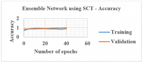
8. When SCT and NCT datasets are used, 3840 SCT and 1792 NCT slices are meant for training. 960 SCT and 448 NCT slices are meant for validation. Ensemble architecture using these datasets is given in Eq. (7). Figure 16 shows the ensemble networks accuracy plot when SCT slices are used.
[Ensemble architecture] s(SCT,NCT) =[Training, Testing and Validation](SCT,NCT) (7)
Once training is over, testing and validation of the datasets are done by the Ensemble network to classify the input slice as PCT, SCT or NCT.
9. The network outputs are connected to the meta learner which is a decision-making model given in Eq. (8). This decision-making model is a voting mechanism.
Figure 16. Accuracy plot of Ensemble network using SCT
Meta learner[Input]=[ (VGG16)Output, (ResNet50)Output, (InceptionV3)Output] (8)
The decision-making model is a technique that monitors the benefits of VGG16, ResNet50, and InceptionV3. Meta learner picks the prediction with the highest number of votes. The working mechanism of the meta learner conforms to the following rules:
10. In the above-explained way the classification is done for the given input shown in Eq. (9).
Output=Classification(Any two or all the three networks decisions) (9)
11. The classification accuracy obtained using an Ensemble network is 74%, 81.98% and 93.76% when PCT, a combination of PCT, SCT and SCT alone are used respectively and compared with the other authors’ work.
Hence, this proposed Ensemble method accurately classifies the normal and abnormal CT images. This deep learning approach classifies the SCT and PCT slices as abnormal CT slices. The model selector is the cause of this gain since it improves network performance by precisely selecting the network that can deliver the best inference for a particular data instance. Table 3 shows the proposed Ensemble architecture classification accuracy, which is compared with various authors’ work.
Table 3. Compared classification accuracy
|
S.No |
Source |
Classification accuracy in percentage |
|
1 |
Anjali Gautam et al (2021) |
92.22 |
|
2 |
Shuo Zhang et al. (2022) |
60.20 |
|
3 |
Glori Stephani Saranih et al. (2020) |
90.666 |
|
4 |
Proposed method |
Using SCT slices alone is 93.76. Using SCT and PCT slices is 81.98. Using PCT slices alone is 74. |
Only in this research work, CT taken after the immediate arrival of the patient and within the golden period used for classification.
In this CNN-based research work, as a first approach, three networks are validated using the transfer learning approach, when trained using the ImageNet dataset. In the second approach, VGG, ResNet50, and InceptionV3 are the networks trained and tested with PCT and SCT slices for classification. In the third approach, Ensemble architecture is designed to do classification. This deep learning Ensemble approach does classification using SCT and PCT slices. This network also does classification when PCT slices alone are used. This CNN-based Ensemble network classifies the abnormal slices in both SCT and PCT slices.
[1] Kanchana, R., Menaka, R. (2017). A novel approach for characterisation of ischaemic stroke lesion using histogram bin-based segmentation and gray level co-occurrence matrix features. The Imaging Science Journal, 65(2): 124-136. https://doi.org/10.1080/13682199.2017.1295586
[2] Öman, O., Mäkelä, T., Salli, E., Savolainen, S., Kangasniemi, M. (2019). 3D convolutional neural networks applied to CT angiography in the detection of acute ischemic stroke. European Radiology Experimental, 3(1): 1-11. https://doi.org/10.1186/s41747-019-0085-6
[3] Surya, S., Yamini, B., Rajendran, T., Narayanan, K.E. (2021). A comprehensive method for identification of stroke using deep learning. Turkish Journal of Computer and Mathematics Education, 12(7): 647-652.
[4] Barros, R.S., Tolhuisen, M.L., Boers, A.M., et al. (2020). Automatic segmentation of cerebral infarcts in follow-up computed tomography images with convolutional neural networks. Journal of NeuroInterventional Surgery, 12(9): 848-852. http://dx.doi.org/10.1136/neurintsurg-2019-015471
[5] Lucas, C., Kemmling, A., Bouteldja, N., Aulmann, L.F., Madany Mamlouk, A., Heinrich, M.P. (2018). Learning to predict ischemic stroke growth on acute CT perfusion data by interpolating low-dimensional shape representations. Frontiers in Neurology, 9: 989. https://doi.org/10.3389/fneur.2018.00989
[6] Khanh, T.L.B., Baek, B.H., Kim, S.K., Do, L.N., Yoon, W., Park, I., Yang, H.J. (2019). Assessment of ASPECTS from CT scans using deep learning. Journal of Korea Multimedia Society, 22(5): 573-579. https://doi.org/10.9717/kmms.2019.22.5.573
[7] Marbun, J.T., Andayani, U. (2018). Classification of stroke disease using convolutional neural network. Journal of Physics: Conference Series, 978(1): 012092.
[8] Song, T. (2019). Generative model-based ischemic stroke lesion segmentation. arXiv Preprint arXiv:1906.02392. https://doi.org/10.48550/arXiv.1906.02392
[9] Chin, C.L., Lin, B.J., Wu, G.R., Weng, T.C., Yang, C.S., Su, R.C., Pan, Y.J. (2017). An automated early ischemic stroke detection system using CNN deep learning algorithm. In 2017 IEEE 8th International Conference on Awareness Science and Technology (iCAST), pp. 368-372. https://doi.org/10.1109/ICAwST.2017.8256481
[10] Meier, R., Lux, P., Jung, S., et al. (2019). Neural network–derived perfusion maps for the assessment of lesions in patients with acute ischemic stroke. Radiology: Artificial Intelligence, 1(5): e190019. https://doi.org/10.1148/ryai.2019190019
[11] Jung, S.M., Whangbo, T.K. (2020). A deep learning system for diagnosing ischemic stroke by applying adaptive transfer learning. Journal of Internet Technology, 21(7): 1957-1968.
[12] Soun, J.E., Chow, D.S., Nagamine, M., Takhtawala, R.S., Filippi, C.G., Yu, W., Chang, P.D. (2021). Artificial intelligence and acute stroke imaging. American Journal of Neuroradiology, 42(1): 2-11. https://doi.org/10.3174/ajnr.A6883
[13] Woo, I., Lee, A., Jung, S.C., et al. (2019). Fully automatic segmentation of acute ischemic lesions on diffusion-weighted imaging using convolutional neural networks: comparison with conventional algorithms. Korean Journal of Radiology, 20(8): 1275-1284.
[14] Clèrigues, A., Valverde, S., Bernal, J., Freixenet, J., Oliver, A., Lladó, X. (2019). Acute ischemic stroke lesion core segmentation in CT perfusion images using fully convolutional neural networks. Computers in Biology and Medicine, 115: 103487. https://doi.org/10.1016/j.compbiomed.2019.103487
[15] Lee, E.J., Kim, Y.H., Kim, N., Kang, D.W. (2017). Deep into the brain: Artificial intelligence in stroke imaging. Journal of Stroke, 19(3): 277. https://doi.org/10.5853/jos.2017.02054
[16] Arab, A., Chinda, B., Medvedev, G., et al. (2020). A fast and fully-automated deep-learning approach for accurate hemorrhage segmentation and volume quantification in non-contrast whole-head CT. Scientific Reports, 10(1): 1-12. https://doi.org/10.1038/s41598-020-76459-7
[17] Ho, K.C., Speier, W., El-Saden, S., Arnold, C.W. (2017). Classifying acute ischemic stroke onset time using deep imaging features. In AMIA Annual Symposium Proceedings, 2017: 892.
[18] Alis, D., Yergin, M., Alis, C., et al. (2021). Inter-vendor performance of deep learning in segmenting acute ischemic lesions on diffusion-weighted imaging: A multicenter study. Scientific Reports, 11(1): 1-10. https://doi.org/10.1038/s41598-021-91467-x
[19] Lisowska, A., O’Neil, A., Dilys, V., et al. (2017). Context-aware convolutional neural networks for stroke sign detection in non-contrast CT scans. In Annual Conference on Medical Image Understanding and Analysis, pp. 494-505. https://doi.org/10.1007/978-3-319-60964-5_43
[20] Wang, C., Shi, Z., Yang, M., et al. (2021). Deep learning-based identification of acute ischemic core and deficit from non-contrast CT and CTA. Journal of Cerebral Blood Flow & Metabolism, 41(11): 3028-3038. https://doi.org/10.1177/0271678X211023660
[21] Gautam, A., Raman, B. (2021). Towards effective classification of brain hemorrhagic and ischemic stroke using CNN. Biomedical Signal Processing and Control, 63: 102178. https://doi.org/10.1016/j.bspc.2020.102178
[22] Suberi, A.A.M., Zakaria, W.N.W., Tomari, R., Nazari, A., Mohd, M.N.H., Fuad, N.F.N. (2019). Deep transfer learning application for automated ischemic classification in posterior fossa CT images. International Journal of Advanced Computer Science and Applications, 10(8): 459-465. https://pdfs.semanticscholar.org/8ce8/e14bdafa25da03cd27d311fbe754ef1b9577.pdf.
[23] Saragih, G.S., Rustam, Z., Aldila, D., Hidayat, R., Yunus, R.E., Pandelaki, J. (2020). Ischemic stroke classification using random forests based on feature extraction of convolutional neural networks. International Journal on Advanced Science, Engineering and Information Technology, 10(5): 2177-2182. https://pdfs.semanticscholar.org/6637/5f983ac274f482c379431d5ec989ad273d15.pdf.
[24] Pereira, D.R., Reboucas Filho, P.P., de Rosa, G.H., Papa, J.P., de Albuquerque, V.H.C. (2018). Stroke lesion detection using convolutional neural networks. In 2018 International Joint Conference on Neural Networks (IJCNN), pp. 1-6. https://doi.org/10.1109/IJCNN.2018.8489199
[25] Zhu, G., Jiang, B., Chen, H., et al. (2020). Artificial intelligence and stroke imaging: A west coast perspective. Neuroimaging Clinics, 30(4): 479-492. https://doi.org/10.1016/j.nic.2020.07.001
[26] Zhang, S., Zhang, M., Ma, S., Wang, Q., Qu, Y., Sun, Z., Yang, T. (2021). Research progress of deep learning in the diagnosis and prevention of stroke. BioMed Research International, 2021. https://doi.org/10.1155/2021/5213550
[27] Yu, Y., Xie, Y., Thamm, T., et al. (2021). Tissue at risk and ischemic core estimation using deep learning in acute stroke. American Journal of Neuroradiology, 42(6): 1030-1037. https://doi.org/10.3174/ajnr.A7081
[28] Rajinikanth, V., Aslam, S.M., Kadry, S. (2021). Deep learning framework to detect ischemic stroke lesion in brain MRI slices of Flair/DW/T1 modalities. Symmetry, 13(11): 2080. https://doi.org/10.3390/sym13112080
[29] Park, S., Kim, B.K., Han, M.K., Hong, J.H., Yum, K.S., Lee, D.I. (2021). Deep learning for prediction of mechanism in acute ischemic stroke using brain MRI.
[30] Chen, Z., Li, Q., Li, R., et al. (2021). Ensemble learning accurately predicts the potential benefits of thrombolytic therapy in acute ischemic stroke. Quantitative Imaging in Medicine and Surgery, 11(9): 3978. https://doi.org/10.21037/qims-21-33
[31] Zhang, S., Wang, J., Pei, L., et al. (2022). Interpretable CNN for ischemic stroke subtype classification with active model adaptation. BMC Medical Informatics and Decision Making, 22(1): 1-12. https://doi.org/10.1186/s12911-021-01721-5
[32] Bhatele, K.R., Bhadauria, S.S. (2020). Glioma segmentation and classification system based on proposed texture features extraction method and hybrid ensemble learning. Traitement du Signal, 37(6): 989-1001. https://doi.org/10.18280/ts.370611