Shuhua Xu | Mingming Qi | Xianming Wang | Hanli Zhao | Zhongyi Hu | Hongyu Sun*
© 2022 IIETA. This article is published by IIETA and is licensed under the CC BY 4.0 license (http://creativecommons.org/licenses/by/4.0/).
OPEN ACCESS
Recently, the generative adversarial network (GAN) has been widely used to obtain the real high-frequency details of images. This spurs the application of GAN in super-resolution reconstruction. However, GAN is unstable in the training process, for the following two reasons: Firstly, the discriminator in GAN keeps the positive (true) and negative (false) criteria of the generated samples unchanged throughout the learning process, without considering the gradual quality improvement of the generated samples (Sometimes, the generated samples are even more realistic than the real samples). To solve the above problems, this paper proposes a super-resolution model based on positive-unlabeled (PU)-GAN-Charbon (SRPUGAN-Charbon). The proposed model includes one generator network that synthetizes super-resolution images and one discriminator network trained to distinguish super-resolution images from real high-resolution images. In addition, the Charbonnier loss function was called to handle the outliers in super-resolution images, and retain the low-frequency features of super-resolution images. Extensive experiments were conducted on three benchmark databases, including BSDS500, Set5, and Set14. The results show that the proposed SRPUGAN-Charbon method is superior to the most advanced methods in terms of visual effect, peak signal-to-noise ratio (PSNR), and structural similarity (SSIM).
positive-unlabeled generative adversarial network (PUGAN), super-resolution reconstruction, charbonnier loss, robustness
High-resolution images, which are rich in texture details, have gained popularity in many fields, such as remote sensing, medical imaging, safety monitoring, and various visual scenes (e.g., industrial scene). The super-resolution reconstruction of high-resolution images from low-resolution images is a typical ill-posed problem.
Recent studies have proved the superiority of convolutional neural network (CNN) in super-resolution reconstruction of high-resolution images [1-3]. In many CNN-based super-resolution methods, the pixel loss is adopted to find the quantitative training indices that improve the peak signal-to-noise ratio (PSNR). Although it can be optimized easily, the pixel loss rarely provides gratifying real details in the light of perceptual vision, which distorts the reconstructed image. The distortion is particularly severe for big scaling factors.
The generative adversarial network (GAN) [4, 5] performs well in generating realistic images, providing a new method for perceptual super-resolution imaging. Ledig et al. [6] attempted to minimize perceptual loss and adversarial loss, and used 16 depth residual blocks and sub-pixel convolution layers to deal with one big scaling factor (×4). Their attempts significantly improved the rich visual perception. However, the GAN-based super-resolution methods have such defects as vanishing gradients, mode collapse, and optimization difficulty in GAN training. As a result, these methods are more likely to collapse quickly, and suffer from over-fitting than CNN-based super-resolution methods [7, 8].
To overcome the above defects, Öcal and Özbakır [9] introduced supervised learning into neural networks. But supervised learning requires a huge amount of training data. To reduce the dependence on numerous training data, Zuo et al. [10] implemented the automatic encoder (AE) in neural network design to learn data feature automatically, and obtain the representation space of low-dimensional potential data. In addition, GAN was combined with AE into a new hybrid generation model to reconstruct high-dimensional data. Nevertheless, there is a contradiction between the fidelity and variety of the potential data representation.
To balance fidelity with variety, Brock et al. [11] applied orthogonal regularization to the generator, making it applicable to simple truncation. Then, the trade-off between sample fidelity and variety could be finetuned by truncating the latent space. Yet this strategy needs a careful design of the network architecture. To avoid the problem, Arjovsky et al. [12] and Gulrajani et al. [13] tried to stabilize the generation process by fitting and optimizing the Wasserstein distance. Miyato et al. [14] proved the necessity and benefits of introducing Lipschitz continuity into the discriminator.
Overall, the existing single image super-resolution methods are unable to deal with multiple degradation well, and poor in generalization. The generated images are often blurry and over smooth. To realize the super-resolution reconstruction of multiple degradation, Lin et al. [15] fully utilized the prior knowledge of fuzzy kernel and noise level in the generation network, employed three discriminators of different scales to reconstruct image details, and thereby maintained the global consistency of the reconstructed image.
The loss functions of the above methods lack texture-oriented optimization, failing to completely maintain the structural information of geometric texture. To improve the perceptual quality of reconstructed images, some researchers regarded regularization as the ultimate solution, the most popular of which is total variation [16-18]. In the context of images, total variation is based on the following fact: an image with excessive and possible false contents, such as noise and unusual artifacts, has a high total variation. This brings an extremely high absolute gradient of the image. The total variation must be minimized to restore the original high-resolution image. In this way, the key features of an image, namely, edges and contours, can be retained, while removing the unnecessary details. Albeit the above strengths, total variation regularization has the following disadvantages: Firstly, false edges often appear in highly noisy images. Secondly, the edges with obvious curvature may be oversmoothed, and the small-scale features may be destroyed. Thirdly, the contrast ratio and geometry structure of the final output may get lost [19].
Perona and Malik [20] proposed another regularization method based on diffusion process: the diffusion rate in the image region is controlled spatially, using a diffusion coefficient. Hence, the outliers are removed without losing the important details of the image. The main shortcomings of the method are as follows: Their flux function is nonmonotonic and not completely convex. Theoretically, uncontrolled non-monotonic and non-convex functions are unstable, which may lead to infinite solutions about the initial image [21, 22]. Charbonnier et al. [23] proposed an alternative flux function that is always monotonic and convex. In practice, their function achieves better results than the Pernoma-Malik method with speckle effect. Zhang et al. [24] developed an enhanced Laplace pyramid network, and trained the network with multilevel CGAN, VGG and robust Charbonnier loss function, producing high-quality super resolution results. Ketsoi et al. [25] improved the feature pyramid network into the enhanced feature block network (EFBN), which adopts high-dimensional feature maps, and uses shared parameters among low-level feature maps. In this way, the computational complexity is reduced, and the perceived quality is improved for the reconstructed images.
At present, the discriminators of SRGAN methods regard the real data as positive samples, and the generated data as negative samples. The discrimination standard remains fixed throughout the training, without considering the gradual quality improvement of the generated data. In fact, the generated data may surpass the real data in terms of quality, making the training unstable. The trained discriminator should neither be too good nor be too bad. Excessively well training will lead to vanishing gradients, and excessively poor training will make it difficult to distinguish between good and bad generated samples. Ideally, the discriminator should be trained to the correct state, which is no easy task in training. What is worse, common measures like PSNR and SSIM are not suitable for measuring the perceptual similarity acceptable to human vision.
To stabilize the discriminator training and ensure the visually perceptibility of reconstructed images, this paper utilizes the positive unlabeled GAN for single image super-resolution reconstruction using a Charbonnier loss function. The main contributions of this paper are as follows:
(1) Taking the Charbonnier penalty function as the loss function, the discriminator was designed to improve the training stability.
(2) The generated super-resolution images were processed as unlabeled samples, making the generator focus on improving the low-quality generated super-resolution images. This improves the performance of the generator.
(3) The real texture, background, and outline details of the reconstructed image were enhanced as much as possible by a new set of perceptual loss, i.e., the weighted sum of content loss, feature loss, texture loss and Charbonnier relative adversarial loss.
2.1 PUGAN
Guo et al. [26] adopted discriminator to process high-quality generated samples as real data, focusing on the generated low-quality samples. The discriminator needs to learn how to distinguish between high- and low- quality samples. Under the guidance of real samples, high-quality samples are identified from the generated samples. This task bears a high resemblance to the positive-unlabeled classification problem [27-29]. Thus, the discriminator is properly trained to the correct state. The trained discriminator is neither too good or too bad, and realizes a high stability. The general framework of PUGAN can be expressed as:
$\max _{\mathrm{G}} \min _{\mathrm{D}} \ell(\mathrm{D}, \mathrm{G})=\pi \mathrm{E}_{\mathrm{P}_{\text {data }}}\left[\mathrm{f}_{1}(\mathrm{D}(\mathrm{x}))\right] +\max \left\{0, \mathrm{E}_{\mathrm{P}_{\mathrm{z}}}\left[\mathrm{f}_{2}(\mathrm{D}(\mathrm{G}(\mathrm{z})))\right]-\pi \mathrm{E}_{\mathrm{P}_{\text {data }}}\left[\mathrm{f}_{2}(\mathrm{D}(\mathrm{x}))\right]\right\}$ (1)
where, $P_{\text {data }}$ is the distribution of real samples; z is the random noise sampled from a priori distribution Pz, i.e., Gaussian distribution; D(x) is the probability for the discriminator to predict x as real data; $f_{1}(\cdot)$ and $f_{2}(\cdot)$ are the losses of classifying input samples as real samples and generated samples, respectively; π is a priori knowledge, i.e., the proportion of high-quality samples in generated samples.
2.2 A-Charbon adaptive super-resolution reconstruction
Maiseli et al. [30] came up with the a-Charbon adaptive super-resolution reconstruction, which automatically switches the regularization part according to image structure. In addition, the parameter $\alpha$ controlling model selection is automatically determined by the program. The method can be expressed as:
$\partial_{\mathrm{t}} \mathrm{y}=\sum_{\mathrm{k}=1}^{\mathrm{N}}\left(\mathrm{b}_{\mathrm{k}}^{\mathrm{T}} \mathrm{b}_{\mathrm{k}} \mathrm{y}-\mathrm{b}_{\mathrm{k}}^{\mathrm{T}} \mathrm{x}_{\mathrm{k}}\right)+\gamma_{1} \mathrm{~N} \Upsilon_{\varepsilon}(|\nabla \mathrm{y}|, \nabla \mathrm{y}, \alpha, \mathrm{k})-\gamma_{2} \mathrm{~N}\left(\mathrm{y}-\mathrm{y}_{0}\right)$ (2)
where, y is the estimated high-resolution image; bk is the transformation matrix of distortion, blur and extraction; xk is the sequence of low-resolution images; $\gamma_{1}$ is a regularization parameter; $\gamma_{2}\left(y-y_{0}\right)$ is a fidelity term; $\gamma_{\varepsilon}(\cdot)=\frac{\nabla y}{\left(1+\left[\frac{|\nabla y|}{k}\right]^{\alpha}\right)^{\frac{1}{\alpha+\varepsilon}}}$ is a-Charbon regularization term.
This section details the proposed approach, namely, SRPUGAN-Charbon.
3.1 Objective loss function
The definition of perceptual loss function [31] is crucial to the performance of the generated network. Inspired by SRGAN [32], our object loss function includes content loss and adversarial loss:
$\ell=\ell_{\text {charbon }}+0.008 \ell_{\mathrm{VGG}-\text { charbon }}+2 \times 10^{-6} \ell_{\alpha \text {-charbon }}+10^{-3} \ell_{\mathrm{PU}-\mathrm{Gen}}$ , (3)
where, $\ell_{\text {charbon }}$ is the Charbonnier loss; $\ell_{V G G-c h a r b o n}$ is the improved VGG loss [33]; $\ell_{\alpha-\text { charbon }}$ is the a-Charbon loss; $\ell_{P U-G e n}$ is the adversarial loss.
3.1.1 Content loss
Mean squared error (MSE) is widely used to improve the PSNR of single image super-resolution reconstruction, but it cannot effectively handle outliers. Hence, a robust loss function $\ell_{\text {charbon }}$ was adopted to handle outliers:
$\ell_{\text {charbon }}=\frac{1}{\mathrm{r}^{2} \mathrm{WH}} \sum_{\mathrm{w}=1}^{\mathrm{rW}} \sum_{\mathrm{h}=1}^{\mathrm{rH}} \rho\left(\mathrm{y}_{\mathrm{w}, \mathrm{h}}-\mathrm{G}(\mathrm{x})_{\mathrm{w}, \mathrm{h}}\right)$, (4)
where, r is the upsampling factor; W and H are the width and height of the high-resolution image, respectively; $\rho(m)=\sqrt{m^{2}+\varepsilon^{2}}, \varepsilon=10^{-3}$ is the Charbonnier penalty function [34]; x is the low-resolution image; y is the original high-resolution image.
Ledig et al. [32] successfully introduced VGG loss [33] into super-resolution reconstruction. This loss has been used not only for pixel level loss, but also for perceptual loss. The loss $\ell_{V G G-c h a r b o n}$ can be defined as:
$\ell_{\mathrm{VGG}-\text { charbon }}=\frac{\sum_{\mathrm{w}=1}^{\mathrm{W}_{5,4 \quad}} \sum_{\mathrm{h}=1}^{\mathrm{H}_{5,4 \quad}} \rho\left(\phi_{5,4 \quad}(\mathrm{y})_{\mathrm{w}, \mathrm{h}}-\phi_{5,4}(\mathrm{G}(\mathrm{x}))_{\mathrm{w}, \mathrm{h}}\right)}{\mathrm{W}_{5,4\quad} \mathrm{H}_{5,4\quad}}$ (5)
where, $\phi_{5,4}$ is the feature map obtained after the rectified linear unit (ReLU) of the 4th convolutional layer [35] and before the 5th max pooling layer in VGG19 [33]; $W_{5,4}$ and $H_{5,4}$ are the width and height of the corresponding feature map, respectively.
Further, a-Charbon regularization was adopted to preserve the good, clear and distinguishable local structure (e.g., edges) of the generated image. The regularization term $\ell_{\alpha-\text { charbon }}$ [30] can be defined as:
$\ell_{\alpha \text {-charbon }}=\frac{1}{\mathrm{r}^{2} \mathrm{WH}} \sum_{\mathrm{w}=1}^{\mathrm{rW}} \sum_{\mathrm{h}=1}^{\mathrm{rH}} \frac{\nabla_{\theta_{\mathrm{G}}} \mathrm{G}(\mathrm{x})_{\mathrm{w}, \mathrm{h}}}{\left(1+\left[\frac{\nabla_{\theta_{\mathrm{G}}} \mathrm{G}(\mathrm{x})_{\mathrm{w}, \mathrm{h}}}{\mathrm{k}}\right]^{\alpha}\right)^{\frac{1}{\alpha+\varepsilon}}}$, (6)
where, θG is the parameter of the generator; 0≤α≤2.
3.1.2 Adversarial loss
Referring to SRGAN [32], the authors added the generation loss to the perceptual loss. The aim is to encourage the network to support the solution residing on the natural image manifold by cheating the discriminator. The specific process is as follows: add one unknown class priori [26] penalty term to the generation loss, treat the generated samples as unlabeled, and make the generator focus on improving the low-quality generated samples. In this way, the generated network is optimized effectively to realize better performance.
The adversarial loss can be defined as:
$\ell_{\mathrm{PU}-\mathrm{Gen}}=\frac{1}{\mathrm{n}} \sum_{\mathrm{i}=1}^{\mathrm{n}}\left(\log \left(1-\mathrm{D}\left(\phi\left(\mathrm{y}_{\mathrm{i}}\right), \phi\left(\mathrm{G}\left(\mathrm{x}_{\mathrm{i}}\right)\right)\right)+\varepsilon\right)+\lambda\left[\| \nabla_{\theta_{\mathrm{d}}}\left(\pi \log \left(\mathrm{D}\left(\phi\left(\mathrm{y}_{\mathrm{i}}\right)\right)\right)+\max \left(\begin{array}{c}0, \log \left(\mathrm{D}\left(\phi\left(\mathrm{G}\left(\mathrm{x}_{\mathrm{i}}\right)\right)\right)\right) \\ \left.\left.-\pi \log \left(\mathrm{D}\left(\phi\left(\mathrm{G}\left(\mathrm{x}_{\mathrm{i}}\right)\right)\right)\right)\right)\right) \end{array}\right)\right)\|_{2}-1\right]^{2}\right)$ (7)
where, $\varepsilon=10^{-2}$ is a parameter to prevent the logarithmic term from being zero; θd is the parameter of the discriminator; π is the a priori knowledge of the class, i.e., the proportion of positive data (high-quality data) in unlabeled data; n is the number of training samples; λ is a regularization parameter.
3.2 Network structure
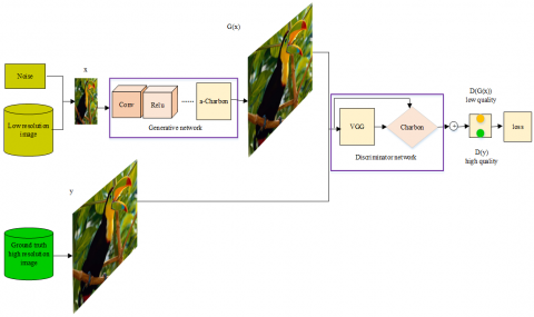
Drawing on the above objective losses, the network structure was determined for our approach (Figure 1).
The proposed approach SRPUGAN-Charbon can be trained in five steps:
Step 1. A low-resolution image x is imported to the generator network, and the good, clear and distinguishable local structure of the generated image is saved by a-Charbon regularization to obtain the corresponding reconstructed image G(x). Then, the content loss between the real high-resolution image y and the reconstructed image G(x) is calculated by Charbon penalty function.
Step 2. The real high-resolution image y and the reconstructed image G(x) are imported into VGG to extract their high-level features, ϕ(y) and ϕ(G(x)). Similarly, the content loss between high-level features ϕ(y) and ϕ(G(x)) is calculated by the Charbon penalty function.
Step 3. The high-level features ϕ(y) and ϕ(G(x)) are inputted into the discriminator network, and the adversarial loss is obtained through PU classification regularization. The final objective loss function is the weighted sum of content loss and adversarial loss.
Step 4. Backpropagation of the network is realized by the adaptive a-Charbon method and PU classification regularization. During the error backpropagation, the gradient of each layer is calculated, and the network is optimized by iteratively updating the discriminator network parameter θd and the generator network parameter θGaccording to the training strategy.
Step 5. The above steps are repeated until the loss function reaches its minimum, marking the end of network training.
Figure 1. Network structure
4.1 Experimental setup
Three extensive benchmark datasets Set5 [36], Set14 [37] and BSDS500 [38] were selected for experiments. In each experiment, the down-sampling factors between super-resolution images and original real images were set to ×2, ×3, and ×4. For comparison, the PSNR and SSIM values of all experiments were calculated on the Y channel of the experimental image. Six super-resolution reconstruction methods were contrasted with our method (SRPUGAN-Charb), including Bicubic, SRResNet [32], SRMD [3], GASRMD [15], ELapCGAN [24] and SREFBN [25].
The low-resolution images were obtained by down-sampling the original high-resolution images with down-sampling factor γ=4. An 84×84 sub-image was cut randomly from each original high-resolution image, and 32 pairs of images were organized into a small batch of data.
Next, the authors set the Adam optimizer [39] with β1=0.9, and initialized the learning rate as 5×10⁻⁵. The discriminator network D and generator network G were alternately trained for 1,000 times to update iteratively. Firstly, generator network G was fixed and the parameters of the discriminator network D were updated through training. Then, discriminator network D was fixed and the parameters of the generator network G were updated through training. In this way, the parameters of D and G were updated alternately until convergence, or reaching the maximum number of iterations. The VGG feature map was configured according to Qiao et al. [40].
4.2 Performance analysis
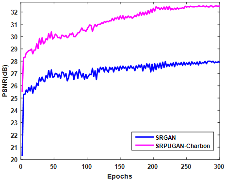
Figure 2 compares the PSNR values of SRGAN [6] and SRPUGAN-Charbon on Set14 test set. With the increase of epochs, the PSNR values of both methods increased. The PSNR values of our model were higher than those of SRGAN.
Figure 2. Comparison between our model and SRGAN on Set14
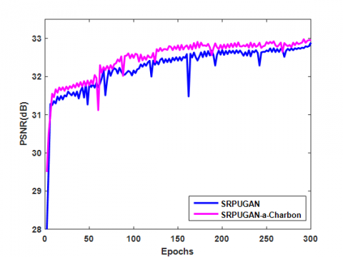
To further improve the performance of reconstructed image, some experiments were carried on the loss function. The a-Charbon loss function was added as one regularization constraint for robust edge preservation. Ten residual blocks were used in the model, and the performance of different methods was compared on Set14. In Figure 3, the red line represents the performance of the model with a-Charbon loss function, while the blue line represents the performance of the model without a-Charbon loss function. It can be seen that the a-Charbon regularization constraint enhanced the performance and stability of the reconstructed image.
Figure 3. Effect of a-Charbon regularization constraint in SRPUGAN on the Set14 test set
4.3 Comparisons with state-of-the-arts
To further showcase the superiority of our SRPUGAN-Charbon, widely controlled experiments were conducted with six state-of-the-arts: Bicubic, SRGAN [32], SRResNet [32], SRMD [3], GASRMD [15], ELapCGAN [24] and SREFBN [25]. The six methods and our method were evaluated on the three benchmark test datasets, using PSNR and SSIM. Tables 1-3 list the comparative results on ×2, ×3 and ×4 SR. Obviously, our SRPUGAN-Charbon method outperformed the six state-of-the-arts.
Moreover, our method was qualitatively compared with the six state-of-the-arts on ×4 SR. Figures 4 and 5 report the reconstruction results of Bicubic, SRResNet, SRMD, GASRMD, ELapCGAN [24] and SREFBN [25], as well as those of our SRPUGAN-Charb. It can be learned that our method recovered more details (e.g., textures), and provided more natural perceived quality than the other methods. The superiority can be attributed to the fact that the generator network in PUGAN focuses on improving the quality of low-quality samples, and that the a-Charbon regularization preserves the good, clear and distinguishable local structure of the generated image, as evidenced by the local enlarged area of reconstructed images in Figures 4 and 5. For example, our method achieved better effects than the contrastive methods in the texture area of bird’s beak, the outer wall behind the foreman, red pepper, the beard around the baboon's mouth, bird’s nest golden straw, and the beak of young bird, and realized higher PSNR and SSIM values than these methods.
Figure 4. Qualitative comparison of our SRPUGAN-Charb and other methods on ×4 SR for 226043 from BSDS500, bird_GT from Set5 and foreman from Set14
Figure 5. Qualitative comparison of our SRPUGAN-Charb and other methods on ×4 SR for Pepper and baboon from Set14, 163004 and 388006 from BSDS500
As shown in Figures 4 and 5, it is clear that GASRMD and SREFBN reconstructed rough image backgrounds: some black spots were added to the running image. On the image of bird’s nest, GASRMD and SREFBN left some strange lines and textures. By contrast, our SRPUGAN-Charb method guaranteed the smoothness of reconstructed image background, and further enhanced the perceived quality of reconstructed images. Consequently, all these experiments proved the robust effects of a-Charbon regularization.
Table 1. Comparison of mean PSNR and SSIM in reconstructed images on three benchmark test sets for scaling factor ×2 using Bicubic, SRResNet, SRMD, GASRMD, ELapCGAN, SREFBN and SRPUGAN-Charbon (ours)
|
Algorithm |
Set5[36] PSNR/SSIM |
Set14 [37] PSNR/SSIM |
BSDS500 [38] PSNR/SSIM |
|
Bicubic |
33.48/0.8307 |
30.25/0.7334 |
28.89/0.6627 |
|
SRResNet |
37.13/0.9113 |
32.78/0.8111 |
30.36/0.7642 |
|
SRMD |
37.35/0.9204 |
32.77/0.8100 |
30.55/0.7905 |
|
GASRMD |
37.39/0.9221 |
32.82/0.8349 |
30.28/0.7441 |
|
ELapCGAN |
37.43/0.9297 |
32.85/0.8516 |
30.57/0.8181 |
|
SREFBN |
37.92 / 0.9593 |
33.59 / 0.9175 |
31.68/ 0.8291 |
|
SRPUGAN-Charbon (ours) |
38.22/0.9602 |
33.68/0.9125 |
31.78/0.8342 |
Table 2. Comparison of mean PSNR and SSIM in reconstructed images on three benchmark test sets for scaling factor ×3 using Bicubic, SRResNet, SRMD, GASRMD, ELapCGAN, SREFBN, and SRPUGAN-Charbon (ours)
|
Algorithm |
Set5 [36] PSNR/SSIM |
Set14 [37] PSNR/SSIM |
BSDS500 [38] PSNR/SSIM |
|
Bicubic |
30.33/0.8211 |
27.57/0.7178 |
26.58/0.6407 |
|
SRResNet |
33.96/0.9017 |
30.10/0.7955 |
28.05/0.7422 |
|
SRMD |
34.20/0.9108 |
30.09/0.7944 |
28.14/0.7685 |
|
GASRMD |
34.22/0.9125 |
30.14/0.8193 |
27.97/0.7221 |
|
ELapCGAN |
34.26/0.9201 |
30.17/0.8360 |
28.26/0.7961 |
|
SREFBN |
34.33/0.9257 |
30.28/0.8407 |
28.56 / 0.8018 |
|
SRPUGAN-Charbon (ours) |
34.54/0.9303 |
30.46/0.8397 |
28.58/0.8021 |
Table 3. Comparison of mean PSNR and SSIM in reconstructed images on three benchmark test sets for scaling factor ×4 using Bicubic, SRResNet, SRMD, GASRMD, ELapCGAN, SREFBN and SRPUGAN-Charbon (ours)
|
Algorithm |
Set5 [36] PSNR/SSIM |
Set14 [37] PSNR/SSIM |
BSDS500 [38] PSNR/SSIM |
|
Bicubic |
28.42/0.8104 |
26.00/0.7027 |
25.36/0.6234 |
|
SRResNet |
32.05/0.8910 |
28.53/0.7804 |
26.83/0.7249 |
|
SRMD |
32.29/0.9001 |
28.52/0.7793 |
27.02/0.7512 |
|
GASRMD |
32.31/0.9018 |
28.57/0.8042 |
26.75/0.7048 |
|
ELapCGAN |
32.35/0.9094 |
28.60/0.8202 |
27.01/0.7788 |
|
SREFBN |
32.38/0.9104 |
28.72/0.8209 |
27.04/0.7802 |
|
SRPUGAN-Charbon (ours) |
32.43/0.9122 |
28.75/0.8236 |
27.08/0.7837 |
This paper proposes a PUGAN-Charbon-based single image super-resolution reconstruction method. Our method includes a generator network for producing super-resolution images, and a discriminator network for judging quality of the generated super-resolution images. The PUGAN model is adopted in the discriminator network to encourage the generator to produce better images, by judging whether the quality of the generated image is good or bad, rather than whether the generated image is from super-resolution image or real high-resolution image. Compared with other GAN models, the PUGAN model enhances the stability of GAN training. To reconstruct the low-frequency and high-frequency features of the low-resolution image, the authors synthetized content loss, adversarial loss and Charbonnier loss into the objective function. Content loss and adversarial loss are conducive to reconstructing the high-frequency features of the low-resolution image, such as textures and edge details, while Charbonnier loss helps to reconstruct the low-frequency features of the low-resolution image, such as image contour and background, by removing outliers. Extensive experiments on three benchmark databases show the advantages of the proposed SRPUGAN-Charbon method over other state-of-the-arts, as indicated by the perceived quality, PSNR and SSIM of reconstructed images.
This work was supported by the Natural Science Foundation of Zhejiang Province under Grants No.: LGG22F020040, LZ21F020001, and LD21F020001, National Social Science Foundation of China under Grant No.: 19BTJ031, the Project of Wenzhou Key Laboratory Foundation under Grant No.: 2021HZSY0071, the Key scientific and technological innovation projects of Wenzhou science and technology plan under Grant No.: ZY2019020, Shandong Provincial Natural Science Foundation under Grant No.: ZR2020MF014.
[1] Wang, Z., Chen, J., Hoi, S.C. (2020). Deep learning for image super-resolution: A survey. IEEE Transactions on Pattern Analysis and Machine Intelligence, 43(10): 3365-3387. https://doi.org/10.1109/TPAMI.2020.2982166
[2] Yang, W., Zhou, F., Zhu, R., Fukui, K., Wang, G., Xue, J.H. (2019). Deep learning for image super-resolution. Neurocomputing, 398: 291-302. https://doi.org/10.1016/j.neucom.2019.09.091
[3] Zhang, K., Zuo, W., Zhang, L. (2018). Learning a single convolutional super-resolution network for multiple degradations. In Proceedings of the IEEE Conference on Computer Vision and Pattern Recognition, pp. 3262-3271.
[4] He, J., Zheng, J., Shen, Y., Guo, Y., Zhou, H. (2020). Facial image synthesis and super-resolution with stacked generative adversarial network. Neurocomputing, 402: 359-365. https://doi.org/10.1016/j.neucom.2020.03.107
[5] Sharma, N., Sharma, R., Jindal, N. (2020). An improved technique for face age progression and enhanced super-resolution with generative adversarial networks. Wireless Personal Communications, 114(3): 2215-2233. https://doi.org/10.1007/s11277-020-07473-1
[6] Ledig, C., Theis, L., Huszár, F., Caballero, J., Cunningham, A., Acosta, A., Shi, W. (2017). Photo-realistic single image super-resolution using a generative adversarial network. In Proceedings of the IEEE Conference on Computer Vision and Pattern Recognition, pp. 4681-4690.
[7] Wu, Z., He, C., Yang, L., Kuang, F. (2021). Attentive evolutionary generative adversarial network. Applied Intelligence, 51(3): 1747-1761. https://doi.org/10.1007/s10489-020-01917-8
[8] Fu, Y., Gong, M., Yang, G., Wei, H., Zhou, J. (2021). Evolutionary GAN-Based Data Augmentation for Cardiac Magnetic Resonance Image. CMC-Computers Materials & Continua, 68(1): 1359-1374.
[9] Öcal, A., Özbakır, L. (2021). Supervised deep convolutional generative adversarial networks. Neurocomputing, 449: 389-398. https://doi.org/10.1016/j.neucom.2021.03.125
[10] Zuo, Z., Zhao, L., Li, A., Wang, Z., Chen, H., Xing, W., Lu, D. (2022). Dual distribution matching GAN. Neurocomputing, 478: 37-48. https://doi.org/10.1016/j.neucom.2021.12.095
[11] Brock, A., Donahue, J., Simonyan, K. (2018). Large scale GAN training for high fidelity natural image synthesis. arXiv preprint arXiv:1809.11096. https://doi.org/10.48550/arXiv.1809.11096
[12] Arjovsky, M., Chintala, S., Bottou, L. (2017). Wasserstein generative adversarial networks. In International Conference on Machine Learning, pp. 214-223.
[13] Gulrajani, I., Ahmed, F., Arjovsky, M., Dumoulin, V., Courville, A.C. (2017). Improved training of wasserstein gans. Advances in Neural Information Processing Systems, 30: 5767-5777.
[14] Miyato, T., Kataoka, T., Koyama, M., Yoshida, Y. (2018). Spectral normalization for generative adversarial networks. arXiv preprint arXiv:1802.05957. https://doi.org/10.48550/arXiv.1802.05957
[15] Lin, H., Fan, J., Zhang, Y., Peng, D. (2020). Generative adversarial image super‐resolution network for multiple degradations. IET Image Processing, 14(17): 4520-4527. https://doi.org/10.1049/iet-ipr.2020.1176
[16] Rudin, L.I., Osher, S., Fatemi, E. (1992). Nonlinear total variation based noise removal algorithms. Physica D: nonlinear phenomena, 60(1-4): 259-268. https://doi.org/10.1016/0167-2789(92)90242-F
[17] Goldstein, T., Osher, S. (2009). The split Bregman method for L1-regularized problems. SIAM Journal on Imaging Sciences, 2(2): 323-343. https://doi.org/10.1137/080725891
[18] Getreuer, P. (2012). Rudin-Osher-Fatemi total variation denoising using split Bregman. Image Processing on Line, 2: 74-95. https://doi.org/10.5201/ipol.2012.g-tvd
[19] Tang, L., Ren, Y., Fang, Z., He, C. (2019). A generalized hybrid nonconvex variational regularization model for staircase reduction in image restoration. Neurocomputing, 359: 15-31. https://doi.org/10.1016/j.neucom.2019.05.073
[20] Perona, P., Malik, J. (1990). Scale-space and edge detection using anisotropic diffusion. IEEE Transactions on Pattern Analysis and Machine Intelligence, 12(7): 629-639. https://doi.org/10.1109/34.56205
[21] Perona, P., Shiota, T., Malik, J. (1994). Anisotropic diffusion. In Geometry-Driven Diffusion in Computer Vision, 73-92. https://doi.org/10.1007/978-94-017-1699-4_3
[22] Höllig, K. (1983). Existence of infinitely many solutions for a forward backward heat equation. Transactions of the American Mathematical Society, 278(1): 299-316. https://doi.org/10.1090/S0002-9947-1983-0697076-8
[23] Charbonnier, P., Blanc-Feraud, L., Aubert, G., Barlaud, M. (1994). Two deterministic half-quadratic regularization algorithms for computed imaging. In Proceedings of 1st International Conference on Image Processing, 2: 168-172. https://doi.org/10.1109/ICIP.1994.413553
[24] Zhang, X., Song, H., Zhang, K., Qiao, J., Liu, Q. (2020). Single image super-resolution with enhanced Laplacian pyramid network via conditional generative adversarial learning. Neurocomputing, 398: 531-538. https://doi.org/10.1016/j.neucom.2019.04.097
[25] Ketsoi, V., Raza, M., Chen, H., Yang, X. (2022). SREFBN: Enhanced feature block network for single‐image super‐resolution. IET Image Processing. https://doi.org/10.1049/ipr2.12546
[26] Guo, T., Xu, C., Huang, J., Wang, Y., Shi, B., Xu, C., Tao, D. (2020). On positive-unlabeled classification in GAN. In Proceedings of the IEEE/CVF Conference on Computer Vision and Pattern Recognition, pp. 8385-8393.
[27] Du Plessis, M.C., Niu, G., Sugiyama, M. (2014). Analysis of learning from positive and unlabeled data. Advances in Neural Information Processing Systems, 27.
[28] Kiryo, R., Niu, G., Du Plessis, M.C., Sugiyama, M. (2017). Positive-unlabeled learning with non-negative risk estimator. Advances in Neural Information Processing Systems, 30.
[29] Xu, Y., Xu, C., Xu, C., Tao, D. (2017). Multi-Positive and Unlabeled Learning. In IJCAI, 3182-3188.
[30] Maiseli, B., Liu, Q., Elisha, O.A., Gao, H. (2013). Adaptive Charbonnier superresolution method with robust edge preservation capabilities. Journal of Electronic Imaging, 22(4): 043027. https://doi.org/10.1117/1.JEI.22.4.043027
[31] Johnson, J., Alahi, A., Li, F.F. (2016). Perceptual losses for real-time style transfer and super-resolution. In European Conference on Computer Vision, 694-711. https://doi.org/10.1007/978-3-319-46475-6_43
[32] Ledig, C., Theis, L., Huszar, F., Caballero, J. (2017). Photo-Realistic Single Image Super-Resolution Using a Generative Adversarial Network. 2017 IEEE/CVF Conference on Computer Vision and Pattern Recognition (CVPR). Honolulu, HI, USA.
[33] Simonyan, K., Zisserman, A. (2014). Very deep convolutional networks for large-scale image recognition. arXiv preprint arXiv:1409.1556. https://doi.org/10.48550/arXiv.1409.1556
[34] Bruhn, A., Weickert, J., Schnörr, C. (2005). Lucas/Kanade meets Horn/Schunck: Combining local and global optic flow methods. International Journal of Computer Vision, 61(3): 211-231. https://doi.org/10.1023/B:VISI.0000045324.43199.43
[35] He, K., Zhang, X., Ren, S., Sun, J. (2015). Delving deep into rectifiers: Surpassing human-level performance on imagenet classification. In Proceedings of the IEEE International Conference on Computer Vision, pp. 1026-1034.
[36] Bevilacqua, M., Roumy, A., Guillemot, C., Alberi-Morel, M.L. (2012). Low-complexity single-image super-resolution based on nonnegative neighbor embedding.
[37] Zeyde, R., Elad, M., Protter, M. (2010). On single image scale-up using sparse-representations. In International Conference on Curves and Surfaces, pp. 711-730.
[38] Martin, D., Fowlkes, C., Tal, D., Malik, J. (2001). A database of human segmented natural images and its application to evaluating segmentation algorithms and measuring ecological statistics. In Proceedings Eighth IEEE International Conference on Computer Vision. ICCV 2001, 2: 416-423. https://doi.org/10.1109/ICCV.2001.937655
[39] Kingma, D.P., Ba, J. (2014). Adam: A method for stochastic optimization. arXiv preprint arXiv:1412.6980. https://doi.org/10.48550/arXiv.1412.6980
[40] Qiao, J., Song, H., Zhang, K., Zhang, X., Liu, Q. (2019). Image super‐resolution using conditional generative adversarial network. IET Image Processing, 13(14): 2673-2679. https://doi.org/10.1049/iet-ipr.2018.6570