Peng Wu | Lu Feng* | Haibo Tong | Zhuxian Zhang
© 2022 IIETA. This article is published by IIETA and is licensed under the CC BY 4.0 license (http://creativecommons.org/licenses/by/4.0/).
OPEN ACCESS
The satellite navigation receiver works in an environment, where the received signal is very weak. Sometimes, frame synchronization is impossible, for the antenna rotates with the flight carrier, and occlusions exist in the environment. After losing look, it is necessary to positioning reacquired signals. Rapid positioning can be completed without frame synchronization, utilizing auxiliary positioning algorithms like A-GPS. If the carrier is highly dynamic, however, the computing load of reacquired signal positioning would be too high, owing to the extreme fuzziness of the approximate position. Therefore, the application of auxiliary positioning algorithms is premised on the acquisition of the approximate position information, when frame synchronization is not possible. This paper proposes a method for estimating the approximate position of a satellite navigation receiver without frame synchronization: The approximate position is quickly obtained by measuring the elevation with a barometer, and searching under a user-defined “geocenter-satellite” coordinate system. Simulation results show that, the proposed algorithm could successfully compute the approximate position, when the barometric altimeter measures elevation with an accuracy within 1.8km, and when the coordinate system is established based on satellites with a long distance and a low angle of elevation, under the condition of global navigation satellite system (GNSS) constellation.
satellite navigation, global navigation satellite system (GNSS), signal transmission time recovery, high dynamics, first positioning time
The satellite navigation receiver needs to receive the signal data through the antenna and other devices to derive the signal time. The signal time above milliseconds are generally acquired after frame synchronization of the received navigation messages. If frame synchronization is impossible, the equivalent calculation of frame synchronization must be completed, assisted by approximate position, approximate time and other information. The auxiliary information is always needed, whether the results of frame synchronization are solved directly from the information, or the frame synchronization is eliminated by auxiliary positioning methods like A-GPS. Approximate information leads to a high accuracy, no matter it is maintained by the crystal oscillator of the receiver, or processed by some time prediction models. On the contrary, the approximate position is easily affected by high dynamics. After the loss of lock, the approximate position is unfeasible due to the large error range.
Domestic research on assisted GPS positioning methods started relatively early [1-5]. In recent years, a series of new methods and new application backgrounds have emerged, which combine relevant algorithms with new disciplines like 5G [7], smart city [8], and artificial intelligence [9]. This trend demonstrates the strong practicality of the assisted GPS positioning algorithms. With the development of society, science, and technology, and the proliferation of various communication infrastructures (e.g., cellular networks and WiFi scenarios), many auxiliary conditions that seemed inconvenient and relevant hardware devices (e.g., portable high-precision clocks) become convenient for data acquisition by the assisted GPS positioning algorithms.
Under weak signal conditions, the receiver is often unable to receive all or part of the messages for bit synchronization, or frame synchronization, making it impossible to acquire the integer part of the milliseconds of the satellite signal transmission time. Then, the positioning cannot be completed by the traditional method [10, 11]. The A-GPS (Assisted-GPS) positioning algorithm sets the receiver millisecond time as the unknown to be solved, and introduces the fifth satellite observation equation to solve the unknown [12-20]. Before operation, the receiver obtains the user’s approximate position, approximate time, and navigation messages via auxiliary methods like information addition, and cellular network reception. After solving the integer part of the milliseconds of receiving signal’s transmission time, the receiver solves the positioning results. The above method is particularly suitable for the weak signal situation. However, the early studies mostly focus on the low dynamic environment, which leads to certain limitations.
In the conventional low-dynamic scenarios of the carrier, the signal reception is generally not blocked or interfered. By contrast, the high-dynamic applications are usually subjected to specific confrontation backgrounds, and highly susceptible to signal interference. Some applications at high altitudes may also be affected by the atmosphere, and thus face short-term loss of lock. The existing algorithms and technical solutions can rely on devices like inertial navigation to mitigate the problem that satellite navigation is susceptible to interference. Nevertheless, the inertial navigation components face a large cumulative deviation, in the absence of satellite navigation. Therefore, it is crucial to restore the capability of satellite navigation as soon as possible when conditions permit. For a highly dynamic aircraft, after the signal is reacquired, the position information before the loss of lock cannot be used as a reference. This is because the high dynamics and other issues could bring a large change in the error of approximate position. The traditional methods will become infeasible due to the large computing load, calling for new algorithms to solve the problem.
When the receiver is near the surface of the earth, the elevation range is about 0~20km, that is, the uncertainty is 10km. The uncertainty is rather small in contrast to the error required to estimate the approximate position of the receiver (no greater than 150km). Thus, the receiver is basically on a sphere near the earth’s surface. Hence, our idea is to establish a polar coordinate system based on two satellites. The coordinates can be represented as a distance and two angles. The distance refers to the elevation of the receiver, and the two angles stand for the position coordinates of the receiver near the ground. In this way, the three-dimensional approximate position of the receiver was reduced to two dimensions.
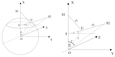
Figure 1. Schematic diagram of user-defined coordinate systemW
In Figure $1, O$ is the center of the earth; $S_{1}$ and $S_{2}$ are two observation satellites. Then, a Cartesian coordinate system was defined, with the geocenter $O$ as the original, and $\overrightarrow{O S_{1}}$ as the $x$-axis direction. The $z$-axis is perpendicular to the plane $\overrightarrow{O S_{1} S_{2}}$, while the y-axis is perpendicular to the plane $\overrightarrow{O X Z}$, and has a right-hand relationship with $X Z$.
Let the receiver position be U, and the delay of the satellite reaching the receiver signal be $\rho_{1}$. Let the distance from a satellite to the geocenter be R, namely, $\overline{O S_{1}}$ and $\overline{O S_{2}}$. Let the angle between the two satellites relative to the geocenter be $\boldsymbol{\tau}$. Let the distance from the receiver to the geocenter be r, namely, $\overrightarrow{O U}$. The value of $\overrightarrow{O U}$ is the sum of the earth radius and the estimated elevation of the receiver. According to the definition of receiver coordinates, the position of the receiver is affected by two angles: field angle $\alpha$ and rotation angle $\gamma$. The former represents the angle between the receiver and the x-axis; the latter refers to the field angle of the receiver on plane OY. In this self-defined coordinate system, the receiver is located near the earth’s surface; r is the known elevation of the receiver; $\alpha$ and $\gamma$are the horizontal coordinates of the receiver. Then, the receiver position can be expressed as $(r, \alpha, \gamma)$.
The ranging values $\rho_{1}$ and $\rho_{2}$ of the two satellites can be respectively calculated by:
${{\rho }_{1}}\left( \alpha \right)=\sqrt{{{R}^{2}}+{{r}^{2}}-2rR\cos \alpha }$ (1)
${{\rho }_{2}}\left( \alpha \gamma \right)=\sqrt{\begin{align} & {{R}^{2}}+{{r}^{2}}-2rR\cos \alpha \cos \tau \\ & -2rR\sin \alpha \sin \tau \cos \gamma \\\end{align}}$ (2)
Specifically, $\alpha$ and $\gamma$ can be determined according to the time in milliseconds of the receiver, and the discrete values of the integer part of the milliseconds. For example, the signal propagation delay from the GPS satellite to the ground is 67~86ms. Then, 20 values of $\alpha$ can be obtained by traversing 20 possible kinds of $\rho_{1}$. Next, 20 possible values of $\gamma$ can be derived from the value of each $\alpha$. In this way, 400 possible combinations between $\alpha$ and $\gamma$ are formed. It is necessary to note a premise: the discretization of $\alpha$ values utilizes auxiliary time. The integer part of the milliseconds are separated by an interval of 1ms. Thus, the auxiliary time should not exceed 0.5ms. Otherwise, more combinations will appear.
The possible error effect should be analyzed before explaining the search for the real approximate position in the user-defined coordinate system.
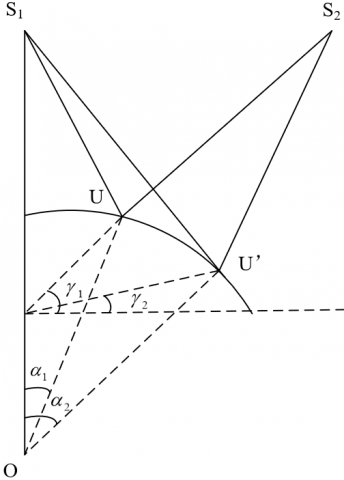
In Figure 2, $\mathrm{U}$ is the real position of the receiver, $(r, \alpha, \gamma)$; $U$ ' is the position to be confirmed due to the error in the auxiliary time, $\left(r, \alpha^{\prime}, \gamma^{\prime}\right)$. The physical interpretation of $U^{\prime}$ is as follows: $r$ is the same for the proximity to the earth's surface. Due to the error in the auxiliary time, the calculated $\alpha$ has deviations, so it is with the $\gamma$ value derived from $\alpha$. The auxiliary time error can be treated as the receiver clock error $\Delta b$.
To analyze the relationship between the clock error $\Delta b$ and the position deviation $\overline{U^{\prime} U}$, the spatial coordinates $(r \cos \alpha$, $r \sin \alpha \cos \gamma, r \sin \alpha \sin \gamma)$ and $\left(r \cos \alpha^{\prime}, r \sin \alpha^{\prime} \cos \gamma^{\prime}\right.$, $\left.r \sin \alpha^{\prime} \sin \gamma^{\prime}\right)$ of $\mathrm{U}$ and $\mathrm{U}^{\prime}$ are derived from the vicinity of the real position $\mathrm{R}$. Then, the direction vector $\overline{U^{\prime} U}$ can be expressed as:
Figure 2. Schematic diagram of proposed approximate position error caused by time error
$\left\{\begin{array}{c}-r \sin \alpha \Delta \alpha \\ r \cos \alpha \cos \gamma \Delta \alpha-r \sin \alpha \sin \gamma \Delta \gamma \\ r \cos \alpha \sin \gamma \Delta \alpha+r \sin \alpha \cos \gamma \Delta \gamma\end{array}\right.$
where, $\Delta \alpha=\alpha_{2}-\alpha_{1} ; \Delta \gamma=\gamma_{2}-\gamma_{1}$.
The two position coordinates of the receiver at U’ corresponding to the ranging values $\rho_{1}^{\prime}$ and $\rho_{2}^{\prime}$ of the two satellites. Under the influence of $\Delta b$, we have:
$\Delta b=\rho_{1}{ }^{\prime}-\rho_{1}=\rho_{2}{ }^{\prime}-\rho_{2}$ (3)
Using formula (1) and its derivable properties, we have
$\Delta b=\rho_{1}^{\prime}-\rho_{1}=\frac{r R \sin \alpha}{\rho_{1}} \Delta \alpha$ (4)
Similarly, using formula (2), we have
$\begin{matrix} \Delta b={{\rho }_{2}}'-{{\rho }_{2}} \\ \begin{align} & =\frac{rR\sin \alpha \sin \tau \sin \gamma }{{{\rho }_{2}}}\Delta \gamma \\ & +\frac{rR\sin \alpha \cos \tau -rR\cos \alpha \sin \tau \cos \gamma }{{{\rho }_{2}}}\Delta \alpha \\\end{align} \\\end{matrix}$ (5)
Combining formulas (4) and (5), it is possible to solve the influence of the local auxiliary time error $\Delta b$ over the error in probability approximate position, i.e., $\Delta \alpha$ and $\Delta \gamma$:
$\left\{ \begin{matrix} \Delta \alpha =\frac{{{\rho }_{1}}}{rR\sin \alpha }\Delta b \\ \Delta \gamma =\frac{{{\rho }_{2}}\Delta b(1-\frac{{{\rho }_{1}}}{{{\rho }_{2}}}\cos \tau +\frac{{{\rho }_{1}}}{{{\rho }_{2}}}\cot \alpha \sin \tau \cos \gamma )}{rR\sin \alpha \sin \tau \sin \gamma } \\\end{matrix} \right.$ (6)
In the rectangular coordinate system, the vector $\overline{U^{\prime} U}$ corresponding to the error direction can be expressed as the following vectors:
$\left\{\begin{aligned} \vec{X}=&-\frac{\rho_{1}}{R} \Delta b \\ \vec{Y}=& \frac{\cos \gamma \cdot \rho_{1}}{R \tan \alpha} \Delta b \\ &-\frac{\rho_{2} \Delta b}{R \sin \tau}\left(1-\frac{\rho_{1}}{\rho_{2}} \cos \tau+\frac{\rho_{1}}{\rho_{2}} \cot \alpha \sin \tau \cos \gamma\right) \\ \vec{Z}=& \frac{\sin \gamma \cdot \rho_{1}}{R \tan \alpha} \Delta b \\ &+\frac{\rho_{2} \Delta b}{R \sin \tau \tan \gamma}\left(1-\frac{\rho_{1}}{\rho_{2}} \cos \tau+\frac{\rho_{1}}{\rho_{2}} \cot \alpha \sin \tau \cos \gamma\right) \end{aligned}\right.$ (7)
Formula (7) shows the effect of $\Delta b$ on the vector: when $\Delta b$ tends to 0 , the size of the vector also tends to 0 . This conforms to the fact that, when $\Delta b$ has no error when establishing the coordinate system, there must be only one true position in the established search space.
To confirm the correctness of the approximate position, the information from other observations needs to be added. Before using the third and more satellites for data redundancy verification, the satellite data, that is, the fractional part of the milliseconds of satellite time, are required.
In the above user-defined coordinate system, the pseudorange measurement equation can be established according to the distance measuring principle of the receiver:
$\Delta {{t}_{i}}=d_{i}^{\left( \alpha ,\gamma \right)}\text{-}\left( d_{i}^{chip}+{{t}_{0}} \right)+\varepsilon _{i}^{pos}+\varepsilon _{i}^{\rho }+\varepsilon _{i}^{{{t}_{0}}}+\varepsilon _{i}^{tro}+\varepsilon _{i}^{sat}$ (8)
where, $\Delta t_{i}$ is the local clock error of the receiver of the i-th verification satellite, which is outside the satellites used to establish the coordinate system; $d_{i}^{(\alpha, \gamma)}$ is the distance of the i-th satellite calculated based on the current position to be confirmed $(\alpha, \gamma) ; \quad d_{i}^{\text {chip }}$ is the fractional part of the milliseconds of pseudoranges measured by the receiver; $t_{0}$ is the auxiliary reception time; $\varepsilon_{i}^{p o s}$ is the clock error induced by the deviations in the line-of-sight vector during the verification of satellite signals, which itself comes from the search error of the receiver for the approximate position arising from the errors in auxiliary time and auxiliary position; $\varepsilon_{i}^{\rho}$ is the error of the original observation information; $\varepsilon_{i}^{t_{0}}$ is the error of the auxiliary time $t_{0} ; \varepsilon_{i}^{\text {tro }}$ is the error of each atmospheric correction value; $\varepsilon_{i}^{s a t}$ is the satellite position error induced by time error, which is reflected as the projection error on the line-of-sight vector.
The original observation information includes three aspects: the fractional measurements in milliseconds of pseudorange results, the auxiliary time, and the auxiliary elevation. Among them, the observation pseudorange accuracy is only affected by the signal strength. As long as the signal can be tracked stably, it is generally within the controllable accuracy range, e.g., within 10m. The auxiliary time is affected by the local clock difference modeling algorithm, the local crystal oscillator accuracy, and the time of losing lock. It can be maintained within 10μs in a short time. As for the auxiliary elevation, some independent sensors can be installed to assist with the elevation measurement. For instance, the barometric altimeter can be adopted for auxiliary elevation measurement. The measurement error of this product can generally be controlled within 100m. Therefore, the error induced by observational measurement is negligible compared to auxiliary time error and auxiliary elevation error.
Figure 3. Influence of the error of the proposed probability position on the ranging values of other verification satellites
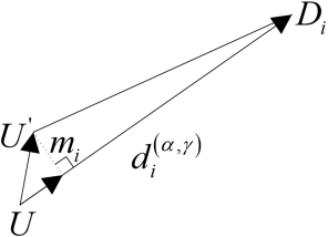
Note that $\varepsilon_{i}^{p o s}$ represents the deviation of the approximate position due to the establishment of the coordinate system, that is, the error caused by $\overline{U^{\prime} U}$. Therefore, it is necessary to analyze the impact of this deviation on other pseudoranges used to verify the calculation. Figure 3 shows the error of the proposed probability position on the ranging values of other verification satellites.
Let $m_{i}$ be the projection of the vector $\overline{U^{\prime} U}$ of the error direction on the line-of-sight vector of the i-th verification satellite $D_{i}$. According to the vector projection formula, the projection can be expressed as:
$m_{i}=\frac{\overrightarrow{U U^{\prime}} \cdot \overrightarrow{U D_{i}}}{\left|\overrightarrow{U D_{i}}\right|}$.
Suppose $\overrightarrow{U D_{l}}=\left(x_{i}, y_{i}, z_{i}\right)$. The projection value is:
$\left|m_{i}\right|=\frac{\rho_{1} \cdot x_{i} \Delta b}{R \cdot d_{i}^{(\alpha, \gamma)}}-\frac{\rho_{1} \cdot\left(\cos \gamma \cdot y_{i}+\sin \gamma \cdot z_{i}\right) \Delta b}{R \tan \alpha \cdot d_{i}^{(\alpha, \gamma)}}$
$+\frac{\Delta b\left(y_{i}-\frac{z_{i}}{\tan \gamma}\right)\left(\rho_{2}-\rho_{1} \cdot \cos \tau+\rho_{1} \cdot \cot \alpha \sin \tau \cos \gamma\right)}{R \sin \tau \cdot d_{i}^{(\alpha, \gamma)}}$ (9)
As shown in formula (9), the presence of $\Delta b$ causes deviation to the approximate location to be confirmed. The deviation, reflected by the vector $\overline{U^{\prime} U}$, eventually influences the pseudoranges of the other satellites in verification. The deviation from the true position is $\left|m_{i}\right|$.
Only from the above conclusion, it is not possible to directly judge which influencing factors cause the increase or decrease of $\left|m_{i}\right|$. But it can be confirmed that when $\Delta b$ tends to 0, this error will also tend to 0, that is, $\varepsilon_{i}^{\text {pos }}$ tends to 0. Therefore, when the auxiliary elevation and time are very accurate, the above-mentioned errors except for the measurement of pseudoranges tend to 0. Therefore, the observation equation can be simplified as:
$\Delta t_{i}=d_{i}^{(\alpha, \gamma)}-\left(d_{i}^{c h i p}+t_{0}\right)$ (10)
By virtue of this conclusion, the above derivation can be verified through experiments and simulations.
Our method only relies on 2 satellites to establish the coordinate system. Their geometric distribution can be easily divided into several simple cases for verification. One factor is the distance between the two satellites, and the other factor is the pitch angle of two satellites. This is easy to understand from the physical principle of geometric distribution. When the time assistance information is already available, the pseudo-satellite at the geocenter derived from the auxiliary elevation, two real satellites, and the receiver form a tetrahedron. The volume of the tetrahedron qualitatively reflects the pros and cons of the geometric distribution. The larger the volume, the better the geometric distribution, the higher the positioning accuracy, and the closer the approximate position to be confirmed is to the real position. The inverse is also true.
The two satellites were selected by their distance, and their pitch angle. Then, the following combinations were configured:
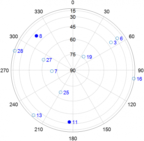
Combination 1: Satellites 11 and 8. These two satellites are far from each other. The connection line between them is in the middle of the sky map, near the zenith.
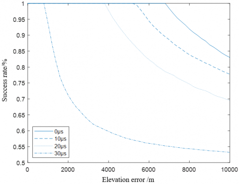
Combination 2: Satellites 11 and 16. These two satellites are far from each other. The connection line between them is at the edge of the star map.
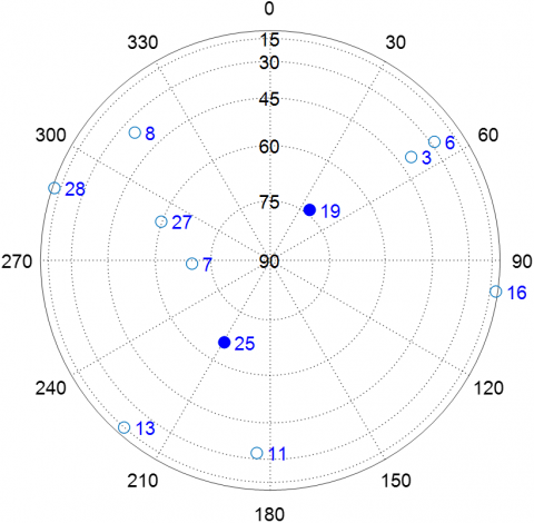
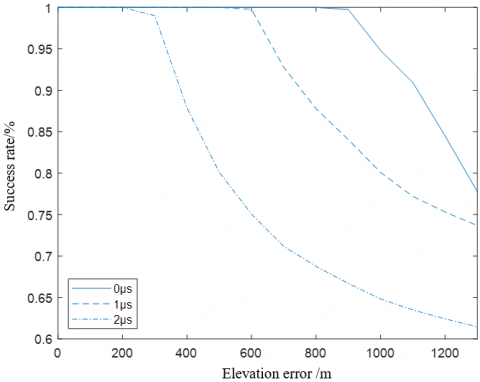
Combination 3: Satellites 19 and 25. These two satellites are close to each other. The connection line between them is in the middle of the sky map, near the zenith.
Figure 4. Distribution and success rate of Combination 1
Figure 5. Distribution and success rate of Combination 2
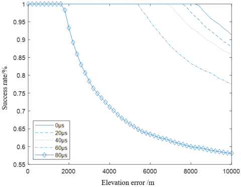
Figure 6. Distribution and success rate of Combination 3
The above Figures 4-6 experimental results suggest that the success rate of the algorithm was affected by the geometric distribution of satellites, which is in line with theoretical expectations. The auxiliary elevation is equivalent to a pseudo-satellite at the geocenter, and the receiver lies right at the middle of the sky map. To improve the geometric distribution of the satellites, it is important to obtain the pitch of the two satellites, and keep the distance between them as large as possible. The above cases show that the success rate of the algorithm could reach 100%, at an elevation error no greater than 1.8km and a time error no greater than 80μs, when the satellite constellation is of high quality, e.g., Satellites 11 and 16 in Combination 2. When the situation was poor, e.g., Satellites 19 and 25 in Combination 3, the elevation error and time error must be controlled to 200m and 2μs, in order to guarantee the success of the algorithm. This limits the application of the algorithm.
When the observation data remain at the same accuracy, the improvement of the geometric distribution of satellites can increase the success rate of the algorithm. From another perspective, to guarantee 100% success rate of the algorithm, it is necessary to choose a better satellite geometric distribution, which relax the accuracy requirements on the auxiliary information. In this way, the application value of the algorithm will be enhanced.
The performance of the algorithm is affected not only by various observational errors, but also by the geometric distribution of satellites. In essence, our algorithm solves positions according to observed quantities. The only difference between it and the traditional algorithm is that: a few results are assumed first, and then verified by substituting more redundant data.
To discretize possible reasonable approximate positions, the algorithm draws on the fact that the integer part of the milliseconds in satellite signal time of A-GPS is unknown, but may be discrete and equally spaced. The auxiliary conditions are utilized to solve the possible integer part of the milliseconds, and derive the positions of all receivers corresponding to the integer part. In this process, the auxiliary time and auxiliary elevation of the two satellites are utilized. The essence is to solve four unknowns from four observation data. Like the traditional theories, the geometric distribution of satellites through the process would affect the final positioning error. In our algorithm, the error directly affects the accuracy of the approximate position to be confirmed. If the positioning error is too large, the position would deviate far from the real approximate position. Then, the positions corresponding to the integer part would be closer to the real positions. All observational data of verification satellites would be affected. In severe cases, the final selection of the approximate position will be incorrect.
This paper proposes a fast estimation algorithm for the approximate position when the receiver cannot complete the frame synchronization. As a supplementation to the traditional A-GPS in high dynamic environment, our algorithm can effectively avoid the failure, when the approximate position cannot be obtained. The adaptability of our algorithm is exceptionally good, because the method is not limited to the type of navigation system or the geographical location. In addition, the authors analyzed the input conditions of the algorithm, and concluded that: as long as the receiver can receive multiple satellites normally, the satellites with better geometric distribution can be selected to form a user-defined coordinate system, and the requirements for auxiliary elevation can be relaxed to obtain an accurate approximate position. In this way, the receiver can complete positioning calculation with a high accuracy.
This paper was supported by Major projects of Changsha Science and Technology Bureau in 2020 (kq2011001), key research and development projects of Hunan Provincial Department of science and technology in 2022 (2022GK2026), Hunan Natural Science Foundation Project (2022JJ30636).
[1] Sirola, N., Syrjärinne, J. (2002). GPS position can be computed without the navigation data. In Proceedings of the 15th International Technical Meeting of the Satellite Division of The Institute of Navigation (ION GPS 2002), Portland, OR, pp. 2741-2744.
[2] Blay, R., Wang, B., Akos, D.M. (2021). Deriving accurate time from assisted GNSS using extended ambiguity resolution. NAVIGATION: Journal of the Institute of Navigation, 68(1): 217-229. https://doi.org/10.1002/navi.412
[3] Aslinezhad, M., Malekijavan, A., Abbasi, P. (2020). ANN-assisted robust GPS/INS information fusion to bridge GPS outage. EURASIP Journal on Wireless Communications and Networking, 2020(1): 129. https://doi.org/10.1186/s13638-020-01747-9
[4] Yang, R., Song, Z., Xi, X. (2019). Self‐assisted first‐fix method for GPS receiver with autonomous short‐term ephemeris prediction. IET Radar, Sonar & Navigation, 13(11): 1974-1980. https://doi.org/10.1049/iet-rsn.2019.0003
[5] Kumar, A., Vohra, M., Prakash, R., Behera, L. (2020). Towards deep learning assisted autonomous UAVs for manipulation tasks in GPS-denied environments. In 2020 IEEE/RSJ International Conference on Intelligent Robots and Systems (IROS), Vegas, NV, USA, pp. 1613-1620. https://doi.org/10.1109/IROS45743.2020.9341802
[6] Xia, J.C., Wang, S.G, Jin, X.N., Zu, G.H., Zeng, Q. (2019). WiFi assisted GNSS positioning with priori geodetic height. Journal of Geomatics, 44(4): 77-82. https://doi.org/10.14188/j.2095-6045.2017221
[7] Gante, J., Sousa, L., Falcao, G. (2020). Dethroning GPS: Low-power accurate 5G positioning systems using machine learning. IEEE Journal on Emerging and Selected Topics in Circuits and Systems, 10(2): 240-252. https://doi.org/10.1109/JETCAS.2020.2991024
[8] López, J.M.L., Aguilar, F.L., Abascal, J.J.C. (2010). A-GPS performance in urban areas. In International Conference on Mobile Multimedia Communications, Lisbon, Portugal, pp. 413-422. https://doi.org/10.1007/978-3-642-35155-6_33
[9] Lim, D.W., Lee, S.J., Cho, D.J. (2007). Design of an assisted GPS receiver and its performance analysis. In 2007 IEEE International Symposium on Circuits and Systems, Orleans, LA, USA, pp. 1742-1745. https://doi.org/10.1109/ISCAS.2007.377931
[10] Li, J. (2010). Eliminating abnormal positioning bias with translation technology in AGPS method. In 2010 The 2nd International Conference on Computer and Automation Engineering (ICCAE), Singapore, pp. 570-574. https://doi.org/10.1109/ICCAE.2010.5451818
[11] Wang, J., Song, M.Z. (2010). Design of a software receiver for GPS weak signal acquisition. Geomatics and Information Science of Wuhan University, 35(7): 846-849. https://doi.org/10.1109/IITA-GRS.2010.5602603
[12] Wei, C.J., Sun, S.L., Jing, X.J., Huang, H. (2010). An enhanced spectrum method for GPS weak signal acquisition. In 2010 Second IITA International Conference on Geoscience and Remote Sensing, Qingdao, China, pp. 502-505. https://doi.org/10.1109/IITA-GRS.2010.5602603
[13] Kazemi, P.L., O’Driscoll, C. (2008). Comparison of assisted and stand-alone methods for increasing coherent integration time for weak GPS signal tracking. In Proceedings of the 21st International Technical Meeting of the Satellite Division of The Institute of Navigation (ION GNSS 2008), Savannah, GA, pp. 1730-1740.
[14] Sahmoudi, M., Amin, M.G., Landry, R. (2008). Acquisition of weak GNSS signals using a new block averaging pre-processing. In 2008 IEEE/ION Position, Location and Navigation Symposium, Monterey, CA, USA, pp. 1362-1372. https://doi.org/10.1109/PLANS.2008.4570124
[15] Bürgi, C., De Mey, E., Orzati, A., Thiel, A. (2006). Highly-integrated solution for ultra-fast acquisition and precise tracking of weak GPS and Galileo L1 signals. In Proceedings of the 19th International Technical Meeting of the Satellite Division of The Institute of Navigation (ION GNSS 2006), Fort Worth, TX, pp. 226-235.
[16] Sirola, N. (2001). A method for GPS positioning without current navigation data. Master of Science Thesis, Tampere University of Technology, Finland.
[17] van Diggelen, F. (2002). Indoor GPS theory & implementation. In 2002 IEEE Position Location and Navigation Symposium (IEEE Cat. No. 02CH37284), Springs, CA, USA, pp. 240-247. https://doi.org/10.1109/PLANS.2002.998914
[18] Dovis, F., Lesca, R., Margaria, D., Boiero, G., Ghinamo, G. (2008). An assisted high-sensitivity acquisition technique for GPS indoor positioning. In Proceedings of IEEE/ION PLANS 2008, Monterey, CA, pp. 1350-1361.
[19] Gong, G., Li, S. (2006). Timing and positioning of assisted-GPS receivers with rough time-tag. International Conference on Space Information Technology, 5985: 931-935. https://doi.org/10.1117/12.658388
[20] Diglys, D. (2010). The use of characteristic features of wireless cellular networks for transmission of GNSS assistance and correction data. In Proceedings of the ITI 2010, 32nd International Conference on Information Technology Interfaces, Cavtat, Croatia, pp. 141-146.