A Novel Approach in Bio-Medical Image Segmentation for Analyzing Brain Cancer Images with U-NET Semantic Segmentation and TPLD Models Using SVM

The term "brain tumour" refers to the uncontrolled growth of brain cells [1]. The two types of tumours are malignant and non-cancerous. In addition to primary and secondary brain tumours, there are many different types of brain tumours that spread from other parts of the body to the brain. Brain tumours are categorised by their size and where they are in the brain. All of these symptoms happen to people who have this condition. They are walking, talking, numbness and sleep are all slowed down by this problem. Most brain tumours don't have a clear reason [2]. The Epstein-Barr virus, ionising radiation, neurofibromatosis, tuberous sclerosis and von Hippel-Lindau syndrome are all examples of rare risk factors. These are some of the more common risk factors: Vinyl chloride, for example, is one example. If you use a cell phone, there isn't enough evidence to say that it is bad for you. Most glial tumours in adults are meningiomas and astrocytoma’s, which are both types of tumours made by cells. Malignant medulloblastoma is the type of cancer that most often affects young people.

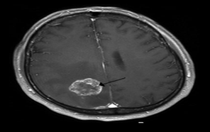
Many times, a CT scan [3] form the Figure 1 and an MRI scan are used together to find out what's wrong with someone health. This happens a lot when someone is getting checked out by a doctor (MRI).

A biopsy is often done to make sure the doctor is right. The information is used to group the tumours based on the severity of the disease. There are a lot of ways to treat this like surgery, radiation and chemotherapy. If there is a seizure, anticonvulsant medicine might be needed to stop it. People who have cancer may need to take dexamethasone [4] and furosemide to cut down on the amount of tumour edoema. In this case, the rate at which the tumour is growing is important. There is now a study of the patient's immune system taking place. Depending on what kind and stage of cancer you have, the prognosis can be very different, and it can also be very good or very bad. Despite the fact that benign tumours only start in one place, their size and where they are important factors in how likely they are to spread. More than a few months after they were diagnosed with GBM (Glioblastoma Multiforme) [5], malignant GBM patients only have about 10% chance of living for more than a few months. There is a good chance that meningiomas that are not cancerous will be able to survive cancer treatment. There are a lot of people in the U.S. who have brain tumours, but most of them live for five years or more. In comparison to secondary or metastatic brain tumours, primary brain tumours happen four times more often than those that spread. People who have lung cancer [6] are behind more than half of all brain tumours that spread from their bodies and reach the brain. A new brain tumour is found in about 250,000 people around the world each year. There are less than 2% of all malignant tumours in the body that are this type of tumour. There are more young people who get a brain tumour than anyone else under the age of 15. People under the age of 15 are most likely to get leukaemia, which is a type of cancer. People who are younger than 15 are most likely to get acute lymphoblastic leukaemia [7].

1.png

Figure 1. A brain CT scans showing the metasis of the cerebral position with annotations from medical image segmentation decathlon

1.1 Research significance in lung cancer segmentation

When cancer is present, it might lead to greater challenges and perhaps death. Since the disease's underlying origins are still unknown, cancer has become more frequent around the world. According to a World Health Organization fact sheet, cancer is the biggest cause of mortality in the world. Cancer will claim the lives of ten million individuals throughout the world in 2020, with the great majority of those deaths happening in low- and middle-income countries. Who would have imagined that lung cancer would be the most common malignancy in the world, with an estimated 2.21 million new cases and 1.80 million fatalities every year. There are a large number of people in attendance. If lung cancer is detected early and treated well, it has the potential to save many lives. The use of technology in the detection of cancer has substantially improved with MRIs, CT scans, X-rays, PET scans, lung biopsies and High-Resolution Computed Tomography (HRCT) being among the most effective (HRCT). The amount of information that can be measured during a clinical CT scan has expanded dramatically as a result of developments in CT technology. For lung segmentation and fusion, computer-aided design (CAD) technology must be linked with computer vision and medical imaging approaches. A critical step in the diagnosis and treatment of a lung condition is the analysis of computed tomography lung images. In this case, it's simple to understand how the pre-processing processes are related to the actual picture generating process in question. As a result, developing more efficient and reliable methods for segmenting CT images of the brain is a fascinating and useful issue to investigate. Lung division may be performed in a variety of methods, the most common of which is by dividing the lung into threshold zones. Among the most critical issues that needed to be solved were the four items listed below:

• The primary goal is to build adaptable bio-medical image analysis technology that can be scaled up quickly in the future.
• The development of tools and strategies for quickly creating ground truth data is the second goal of the project.
• What is the best method of analyzing medical images from a broad variety of data is the third question that has to be addressed for lung cancer segmentation.
• The procedure's progression. Achieving accurate and customised representations of the human anatomy and organs is critical for medical education.

The major contributions of the paper are as follows:

The goal of this study is to devise a method of separating and combining images of the brain. Images may be segmented more quickly using U-NET semantic segmentation and TPLD models that make use of SVMs, both of which are available for free. Saving time is a great approach to improve your productivity. The proposed solution, which has been shown to be fairly efficient in identifying CT scan parts, also makes use of morphological approaches and masking techniques. We were able to greatly speed up computations while preserving accuracy in the most difficult circumstances, and we didn't have to do any post-processing because we used a distributed computing approach. Strategy: The use of SVM image fusion algorithms in conjunction with the three-parameters results in improved outcomes and a more effective technique for the fusion of medical images in the treatment of lung cancer. We took use of three characteristics of the multi-view clinical CT scans in order to expedite the process of building the sub-dictionaries. Brain tumours are difficult to distinguish from one another and researchers can't tell how rough their surfaces are. Artefacts frequently obscure CT [8] can results. Image editing software is required. The research evaluates four aspects of brain magnetic resonance image segmentation and surface texture analysis.

1. Brain imaging is discussed in full.
2. U-Net with three parameters logistic distribution has been demonstrated to greatly enhance brain tumour segmentation accuracy when compared to earlier models. This method is abbreviated U-Net-LD.
3. The Probability Density Function, there are three components in the U-Net structure that must deal with memory and processing constraints, as well as class imbalance.
4. We employed a U-Net, a three-parameter Logistic Distribution and a Support Vector Machine to study brain tumors segmentation and the detailed comparison of various approaches.

This article will provide an outline of current biological image processing research. It will focus on a range of brain cancer abnormalities, suggested U-Net segmentation technologies and hybrid algorithms that integrate parts of exact nodule prediction with spatial imaging processes.

3.1 U-Net architecture

A network called U-Net was used to separate images of cancerous images [14]. It uses a shrinking trail for context and a long straight trail to show where it is. When you choose a route, think about the three convolutional layers. Dropout layers [15] and pooling are also part of this type of stacking. Skip connections are used to connect channels that grow and shrink. Convolutional kernels appear in each of the three layers and there are nine of them in each. Second layer: It has twice as many filters as the first layer. When we did this, we used Adam's method [16] of optimising things and normalising things to do it. The loss function was also cross-entropy-weighted to make sure it was accurate. Finally, the model was ready to go. It had been trained for four iterations at a rate of 0.001.

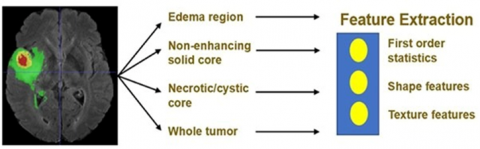
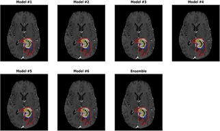
This work came up with an ensemble model that was better at segmenting and had less model variance (see Figure 2). (majority) People learned about a lot of things on their own as part of their training. The model's performance on the validation set was used to figure out how many training runs were needed. In one of the models, each voxel had a class. The majority rule was used to figure out which class each voxel belonged to. These images can show quantitative data about the features of brain tumours. This can help people learn more about them. In addition to the whole tumour, EDOEMOMA has non-enhanced solid cores, necrotic or cystic areas and the whole tumour area. Figure 3 shows the detailed architecture of the proposed architecture.

2.png

Figure 2. Feature extraction of the U-NET architecture

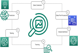
3.1.1 Block diagram of the proposed architecture

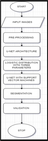
In Figure 3, the steps in our proposed solution for the brain tumour segmentation task are image pre-processing, the extraction of patches, the training of many models using a generic U-Net structure with configurable hyper-parameters and Logistic three parameters. The deployment of each model to predict the full volume of a tumour and the final ensemble phase. The steps in the survival prediction challenge are feature extraction, model fitting, and deploying the model.

3.png

Figure 3. Block diagram of the proposed architecture

3.2 Logistic distribution with three parameters

The logistic type mixture distribution based on three-parameters consist of leptokurtic distribution for specific values of the shape parameter ‘p’. In developing the segmentation model, the most important task is performing the estimation of model parameters. An effective methodology in estimating the parameters of mixture distribution is utilizing Expectation Maximization algorithm. The efficiency of EM algorithm [17] depends on the initial values of the parameters and number of mixture components in the model. K-means algorithm for obtaining initial values of the model parameters. the performance comparison taken by k-means algorithm and hierarchical clustering algorithm; it is required to assign an initial value to the number of image regions. To overcome this disadvantage the hierarchal clustering algorithm is used for obtaining the number of components in the mixture model and initializing the model parameters. In this paper, it is assumed that the pixel intensities of the image regions follow a logistic type distribution based on three-parameters as a result, the whole image is considered by a k-component mixture with logistic type distribution which was based on three parameters. The probability distribution function (P.D.F) [18] of the current model logistic type distribution which was three parameters is given in Eq. (1).

The frequency curves associated with logistic type distribution for three parameters are shown in Figure 4.

$f\left(y, \mu, \sigma^{2}\right)=\frac{\left[\frac{3}{\left(3 p+\pi^{2}\right)} \quad \right]\left[p+\left(\frac{y-\mu}{\sigma}\right)^{2}\right] e^{-\left(\frac{y-\mu}{\sigma}\right)}}{\sigma\left[1+e^{-\left(\frac{y-\mu}{\sigma}\right)} \quad \right]^{2}}$       (1)

where, $-\infty<y<\infty,-\infty<\mu<\infty, p \geq 4$.

4.png

Figure 4. Frequency curve of logistic type distribution with three parameter

The distribution function of the current model with μ and the model is symmetric as,

$F(X)=\frac{3 e^{-\left(\frac{y-\mu}{\sigma}\right)}}{\sigma^{2}\left(12+\pi^{2}\right)}$

$\frac{\left[\left[4+\left(\frac{y-\mu}{\sigma}\right)^{2}\right]\left[2\left(\frac{y-\mu}{\sigma}\right)-1\right] e^{-\left(\frac{y-\mu}{\sigma}\right)^{2}}-\left[\left(\frac{y-\mu}{\sigma}\right)-1\right]^{2}\right]}{\left[1+e^{-\left(\frac{y-\mu}{\sigma}\right)^{2}} \quad \right]^{2}}$       (2)

where, $\mathrm{k}$ is the number of regions $0 \leq \alpha_{i} \leq 1$ are weights such that $\sum \alpha_{i}=1$ and $f_{i}\left(x, \mu, \sigma^{2}\right)$ is given in Eq. (1). $\alpha_{i}$ is the weight associated with i th region in the whole region.

The image region pixel intensities are considered as feature of the image. Here, the logistic type distribution based on three-parameter is assumed for modelling the image region pixel intensities. The probability density function (p.d.f) of the pixel intensities is of the form

$f\left(y, \mu, \sigma^{2}, z\right)=\frac{\left[\frac{3}{\left(3 z+\pi^{2}\right)} \quad \right]\left[z+\left(\frac{y-\mu}{\sigma}\right)^{2}\right] e^{-\left(\frac{y-\mu}{\sigma}\right)}}{\sigma\left[1+e^{-\left(\frac{y-\mu}{\sigma}\right)} \quad \right]^{2}}$       (3)

where, $-\infty<y<\infty,-\infty<\mu<\infty, z \geq 4, \sigma^{2}>0$.

For the whole image, the mean pixel intensity represented as,

$p(y)=\sum_{i=1}^{k} \alpha_{i} f_{i}\left(y, \mu, \sigma^{2}\right)$      (4)

Here $\mathrm{k}$ is the number of regions $0 \leq \alpha_{i} \leq 1$ are weights such that $\sum \alpha_{i}=1$ and $f_{i}\left(y, \mu, \sigma^{2}\right)$ is given in Eq. (1). $\alpha_{i}$ is the weight associated with $i^{\text {th }}$ region in the whole image. The pixel intensities on images are correlated with each other in normal cases. These correlations could be identified and processed with the help of various spatial sampling models like or spatial averaging. For the whole image, the mean of pixel intensity is represented as

$E(X)=\sum_{i=1}^{K} \alpha_{i} \mu_{i}$      (5)

For the current parameter based logistic type distribution, the likelihood equation is nonlinear and there is no solution by analytic means. Consequently, we use some iterative procedure like EM algorithm for obtaining the estimates of the parameters. For Expectation Maximization (EM) algorithm, the updated equations of the model parameters are the likelihood of the function of model is

$L(\theta)=\prod_{S=1}^{N} p\left(x_{s}, \theta^{(l)}\right)$       (6)

$L(\theta)=\prod_{s=1}^{N}\left(\sum_{i=1}^{k} \alpha_{i} f_{i}\left(x_{s}, \theta^{(l)}\right)\right.$      (7)

This implies

$\log L(\theta)=\sum_{S=1}^{N} \log \left(\sum_{i=1}^{k} \alpha_{i} f_{i}\left(x_{s}, \theta^{(l)}\right)\right)$       (8)

where, $\theta=\left(\mu_{i}, \sigma_{i}^{2}, \alpha_{i} ; i=1,2, \ldots \ldots \ldots \ldots \ldots . . k\right)$ is the set of parameters, therefore, three parameter logistic type distribution:

$\log L(\theta)$$=\sum_{S=1}^{N} \log \left[\sum_{i=1}^{m} \alpha_{i} \frac{\left[\frac{3}{\left(3 p+\pi^{2}\right)} \quad \right]\left[p+\left(\frac{x_{s}-\mu_{i}}{\sigma_{i}}\right)^{2}\right] e^{-\left(\frac{x_{s}-\mu_{i}}{\sigma_{i}}\right)}}{\sigma_{i}\left[1+e^{-\left(\frac{x_{s}-\mu_{i}}{\sigma_{i}}\right)} \quad \right]^{2}} \quad \right]$      (9)

The process of estimating the likelihood function on sample observations is considered as the first step of the EM algorithm and is obtained as,

E-STEP: -

In the expectation (E) step, the expectation value of log $L(\theta)$ with respect to the initial parameter vector $\theta^{(0)}$ is

$Q\left(\theta, \theta^{(0)}\right)=E_{\theta^{(0)}}\left[\frac{\log L(\theta)}{\bar{x}}\right]$       (10)

Given the initial parameters $\theta^{(0)}$. One can compute the density of pixel intensity X as

$P\left(x_{s}, \theta^{(l)}\right)=\sum_{i=1}^{k} \alpha_{i} f_{i}\left(x_{s}, \theta^{(l)}\right)$       (11)

$L(\theta)=\prod_{s=1}^{N} p\left(x_{s}, \theta^{(l)}\right)$      (12)

This implies

$\log L(\theta)=\sum_{S=1}^{N} \log \left(\sum_{i=1}^{k} \alpha^{(l)}{ }_{i} f_{i}\left(x_{s}, \theta^{(l)}\right)\right)$       (13)

The provisional likelihood which goes to region ‘k’ is

$P_{k}\left(x_{s}, \theta^{(l)}\right)=\left[\frac{\alpha_{k}^{(l)} f_{k}\left(x_{s}, \theta^{(l)}\right)}{p_{i}\left(x_{s}, \theta^{(l)}\right)}\right]$       (14)

$p_{k}\left(x_{s}, \theta^{(l)}\right)=\left[\frac{\alpha_{k}^{(l)} f_{k}\left(x_{s,} \theta^{(l)}\right)}{\sum_{i=1}^{k} \alpha_{i}^{(l)} f_{i}\left(x_{s}, \theta^{(l)}\right)}\right]$       (15)

For the samples, the log likelihood function is

$Q\left(\theta, \theta^{(l)}\right)=E_{\theta^{(l)}}[\log L(\theta) / \bar{x}]$      (16)

Therefore, for Three parameter logistic type distribution:

$f_{i}\left(x_{s}, \theta^{(l)}\right)$$=\frac{\left[\frac{3}{\left(3 p+\pi^{2}\right)}\right]\left[p+\left(\frac{x_{s}-\mu_{i}^{(l)}}{\sigma^{(l)}}\right)^{2}\right] e^{-\left(\frac{x_{s}-\mu_{i}^{(l)}}{\sigma_{i}^{(l)}}\right)}}{\sigma_{i}^{(l)}\left[1+e^{-\left(\frac{x_{s}-\mu_{i}^{(l)}}{\sigma_{i}^{(l)}}\right)}\right]^{2}}$        (17)

M-STEP: -

In order to get the model parameters estimation, one should increase $Q\left(\theta, \theta^{(l)}\right)$ such that $\sum \alpha_{i}=1$. This estimation could be achieved by using the first order Lagrange type function

$F=\left[E\left(\log L\left(\theta^{(l)}\right)\right)+\beta\left(1-\sum_{i=1}^{k} \alpha_{i}^{(l)}\right)\right]$       (18)

where, $\beta$ is Lagrangian multiplier which combines both the log likelihood functions which needs to be maximized. The two steps mentioned above are repeated based on the necessity which every iteration is used to increase the log likelihood of the model and the model is used to converge with a likelihood function.

The Updated equations of $\alpha_{i}$:

To find the expression for $\alpha_{i}$, we solve the following equation

$\frac{\partial F}{\partial \alpha_{i}}=0$        (19)

$\sum_{i=1}^{N} \frac{1}{\alpha_{i}} P_{i}\left(x_{s}, \theta^{(l)}\right)+\beta=0$       (20)

After adding on both sides, $\beta=-N$.

Therefore,

$\alpha_{i}=\frac{1}{N} \sum_{s=1}^{N} P_{i}\left(x_{s}, \theta^{(l)}\right)$       (21)

The updated equations of $\alpha_{i}$ for $(l+1)^{t h}$ iteration is

$\alpha_{i}^{(l+1)}=\frac{1}{N} \sum_{s=1}^{N} P_{i}\left(x_{s}, \theta^{(l)}\right)$       (22)

This implies

$\alpha_{l}^{(l+1)}=\frac{1}{N} \sum_{s=1}^{N}\left[\frac{\alpha_{l}^{(l)} f_{l}\left(x_{s} \theta^{(l)}\right)}{\sum_{i=1}^{k} \alpha_{i}^{(l)} f_{i}\left(x_{s}, \theta^{(l)}\right)}\right]$      (23)

The Updated equations of $\mu_{i}$ :

For updating the parameter $\mu_{i}, i=1,2,3 \ldots k$, we consider the derivatives of $Q\left(\theta, \theta^{(l)}\right)$ with respect to $\mu_{i}$ and equal to zero, we have

$Q\left(\theta, \theta^{(l)}\right)=E\left[\log L\left(\theta, \theta^{(l)}\right)\right]$      (24)

Therefore, $\frac{\partial}{\partial \mu_{i}}\left(Q\left(\theta, \theta^{(l)}\right)\right)=0$.

Implies

$E\left[\frac{\partial}{\partial \mu_{i}}\left(\log L\left(\theta, \theta^{(l)}\right)\right)\right]=0$       (25)

For Two parameter logistic type distribution:

By applying the derivative with respect to $\mu_{i}$, we have

$\frac{\partial}{\partial \mu_{i}}\left[\sum_{s=1}^{N} \sum_{i=1}^{K} P_{i}\left(y_{s.}, \theta^{l}\right) \log \alpha_{i} \frac{\left[\frac{3}{12+\pi^{2}} \quad \right]\left[4+\left(\frac{y_{s}-\mu_{i}}{\sigma_{i}}\right)^{2}\right] e^{-\left(\frac{y_{s}-\mu_{i}}{\sigma_{i}}\right)}}{\sigma_{i}\left[1+e^{-\left(\frac{y_{s}-\mu_{i}}{\sigma_{i}}\right)^{2}}\right]} \quad \right]=0$     (26)

Since $\mu_{i}$ appears in only one region, $\mathrm{i}=1,2,3 \ldots \mathrm{k}$ (regions), for Three parameter logistic type distribution:

$\frac{\partial}{\partial \mu_{i}}\left[\sum_{s=1}^{N} \sum_{i=1}^{K} P_{i}\left(y_{s.}, \theta^{l}\right) \log \left[\alpha_{i} \frac{\left[\frac{3}{3 p+\pi^{2}} \quad \right]\left[p+\left(\frac{y_{s}-\mu_{i}}{\sigma_{i}}\right)^{2}\right] e^{-\left(\frac{y_{s}-\mu_{i}}{\sigma_{i}}\right)}}{\sigma_{i}\left[1+e^{-\left(\frac{y_{s}-\mu_{i}}{\sigma_{i}}\right)} \quad \right]^{2}} \quad \right]\right]=0$      (27)

Finally, for Three parameter logistic type distribution:

$\mu_{i}^{(l+1)}=\frac{\sum_{s=1}^{n} \frac{P_{i}\left(y_{s.}, \theta^{(l)}\right)\left(2 y_{s}\right)}{\left(\sigma_{i}^{2}\right)^{(l)}\left[p+\left(\frac{y_{s}-\mu_{i}^{(l)}}{\sigma_{i}^{(l)}}\right)^{2}\right]}-\sum_{S=1}^{n} \frac{P_{i}\left(y_{s.}, \theta^{(l)}\right)}{\sigma_{i}^{(l)}}+\sum_{S=1}^{n} \frac{2 P_{i}\left(y_{S .}, \theta^{(l)}\right)}{\sigma_{i}^{(l)}\left[1+e^{\left(\frac{y_{s}-\mu_{i}^{(l)}}{\sigma_{i}^{(l)}}\right)}\right]}}{2 \sum_{s=1}^{n} \frac{P_{i}\left(y_{s.}, \theta^{(l)}\right)}{\left(\sigma_{i}^{2}\right)^{(l)}\left[p+\left(\frac{y_{s}-\mu_{i}^{(l)}}{\sigma_{i}^{(l)}}\right)^{2}\right]}}$       (28)

The updated equation of $\sigma_{i}^{2}$ :

For updating $\sigma_{i}^{2}$ we differentiate $Q\left(\theta, \theta^{(l)}\right)$, that is, $\frac{\partial}{\partial \sigma^{2}}\left(Q\left(\theta, \theta^{(l)}\right)\right)=0$.

This implies

$E\left[\frac{\partial}{\partial \sigma^{2}}\left(\log L\left(\theta, \theta^{(l)}\right)\right)\right]=0$      (29) 

For three parameter logistic type distribution:

$\frac{\partial}{\partial \sigma_{i}^{2}}\left[\sum_{s=1}^{N} \sum_{i=1}^{K} P_{i}\left(y_{s.}, \theta^{l}\right) \log \alpha_{i} \frac{\left[\frac{3}{3 p+\pi^{2}} \quad \right]\left[p+\left(\frac{y_{s}-\mu_{i}}{\sigma_{i}}\right)^{2}\right] e^{-\left(\frac{y_{s}-\mu_{i}}{\sigma_{i}}\right)}}{\sigma_{i}\left[1+e^{-\left(\frac{y_{s}-\mu_{i}}{\sigma_{i}}\right)} \quad \quad \right]^{2}}\right]=0$      (30)

$\sigma_{i}^{2^{(l+1)}}=\frac{\sum_{s=1}^{N} \frac{P_{i}\left(y_{s.} , \theta^{(l)}\right)\left(y_{s}-\mu_{i}^{(l+1)} \quad \right)}{2 \sigma_{i}^{3^{(l)}}} \quad - \quad \sum_{s=1}^{N} \frac{P_{i}\left(y_{s.} , \theta^{(l)}\right)\left(y_{s}-\mu_{i}^{(l+1)} \quad \right)}{\sigma_{i}^{3^{(l)}}\left[1+e^{\frac{\left(x_{s}-\mu_{i}\right)}{\sigma_{i}}}\right]} \quad - \quad \sum_{s=1}^{N} \frac{P_{i}\left(y_{s.} , \theta^{(l)}\right)}{2 \sigma_{i}^{2^{(l)}}}}{\sum_{s=1}^{N} \frac{P_{i}\left(y_{s.} , \theta^{(l)}\right)\left(x_{s}-\mu_{i}^{(l+1)} \quad \right)^{2}}{\sigma_{i}^{4^{(l)}}\left[p \sigma_{i}^{2^{(l)}}+\left(y_{s}-\mu_{i}^{(l+1)} \quad \right)^{2}\right]}}$       (31)

where,

$p_{i}\left(y_{s}, \theta^{(l)}\right)=\left[\frac{\alpha_{i}^{(l+1)} f_{i}\left(y_{s} \mu_{i}^{(l+1)},\sigma_{i}^{2^{(l)}}\right)}{\sum_{i=1}^{k} \alpha_{i}^{(l+1)} f_{i}\left(y_{s}, \mu_{i}^{(l+1)}, \sigma_{i}^{(l)}\right)}\right]$       (32)

3.3 U-NET with support vector machine

Some of the parameters like $\alpha_{i}, \mu$ and $\sigma^{2}$ are typically measured as identified apriori. A normally cast-off technique in preparing limits is through selecting a arbitrary example from the whole image. If the sample size is small, this method works very well, but it fails when the size of the image is big and some of the regions on the images are not identified fully. In order to solve this problem, the K-means algorithm is used such that to break the images in to homogeneous regions. The procedure for the hyperplanes algorithm is as follows,

1. Select Hyperplanes from the dataset as early clusters randomly and these data points considered as centroids in the initial cases.

2. By calculating the Hypertext characterization distance from each cluster to the center of the cluster with data points.

3. Based on the distance value minimum, find the new cluster.

4. Replication of step 2 and 3 until clustering center do not change.

5. End the model implementation.

3.4 Segmentation algorithm

Once the refinement of image parameters process had completed, the important task to be performed in the process of segmentation is the assignment of pixels to the various parts or segments of the image. The process followed in this algorithm is as follows,

Step 1: At first step the histogram of the whole image was plotted.

Step 2: Get the estimates in the initial phases of the model equations by using the Support vector means algorithm for various regions of the whole images.

Step 3: Get the modified estimates of the model.

Step 4: Allocate a piece pixel to conforming jth region based on maximum likelihood of the model were

$L_{j}=M A X\left[\frac{\left[\frac{3}{\left(3 p+\pi^{2} \quad \right)}\right]\left[p+\left(\frac{y_{s}-\mu_{i}}{\sigma_{i}}\right)^{2}\right] e^{-\left(\frac{y_{s}-\mu_{i}}{\sigma_{i}}\right)}}{\sigma_{i}\left[1+e^{-\left(\frac{y_{s}-\mu_{i}}{\sigma_{i}}\right)} \quad \right]^{2}} \quad \right]$,

$-\infty<\mu_{i}<\infty,-\infty<\sigma_{i}^{2}<\infty, p \geq 4$

3.5 Proposed model learning lifecycle

The Proposed Model life cycle was shown in the Figure 5. A detailed process of Pre-Processing, Model Definition and Testing and lastly prediction cycle can be observed.

5.png

Figure 5. Proposed lifecycle of the classifier

5.1 Tumour segmentations and results

A U-Net group was used to separate brain tumours. Networks with different encoding and decoding block counts, patch sizes, and loss weights were trained and put together. The stand-alone models didn't do as well as the group model did. Linear regression was used to combine non-imaging clinical variables like age and resection status with six important characteristics from segmentation labels in order to improve the chances of survival. People who took part in the challenge came up with the most accurate predictions of how long they would live. In order to make a network, we couldn't pick the best model or set of hyper-parameters because their performance was so close. In terms of network design, there isn't a clear winner between dense-net and the U-Net [31-33]. Table 2 showing the model performance of the ablation study on the MISD dataset.

People can't study how DCNN's design and features affect how well the network works because it's a "black box." Models can't be judged because they take a long time to calculate and use questionable validation datasets. Our study used a three-dimensional U-Net to find patches of different sizes. A wide range of architectural styles could be used to make up for a model's flaws. We're trying to balance the amount of time we spend training and testing with how well we think we'll do, just like averages can be used in measurements to improve the signal-to-noise ratio. Table 3 showing the performance of the various classifiers with respective to the MSD.

Figure 8 shows the evaluation of the classifiers, our method doesn't use objective measurements to figure out which model combination is best. This makes it hard to find the best model combination. Instead, there were no models or hyperparameters [34] that were used instead of them. It isn't possible to get around this restriction by not using N-fold cross validation. The validation set (66 occurrences) is a lot smaller than both the training and testing datasets. The U-Net model, on the other hand, predicts the whole input label map, not just the centre pixel. Because the GPU has a limited amount of memory, smaller parts of a picture are deleted when the whole picture is used as an input. It's possible that pixels near the edge of the receptive field have a smaller receptive field because only half of the receptive field is used. Even though, most GPUs can only use 12 GB of RAM. Edge pixels have a smaller receptive field than the rest of the pixels, which can be fixed by setting up a big overlap sliding window deployment. Even though our past research didn't show a big difference between the recommended strategy and the one we used, bias correction was often used during pre-processing. [*] For any intensity-based approach, pre-compensation may not be needed if the DCNN can learn and deal with picture biases, which it can do. We didn't use the bias correction method in our last tests because we didn't have enough time.

8.png

Figure 8. Evaluation of the classifiers

Table 2. Model performance after ablation study on the MISD dataset

Table 3. Performance of the various classifiers with respective to the MISD

This is not the only thing that will be needed for more research in this field. Because we could look at each occurrence individually, the median metrics of the segmentation findings were better than the mean metrics. There was one final model that gave Dice scores of 96%. This one was the best one. People understand why they're worried about dice results that range from 0 to 1. To show how many places it missed, Dice scores for ET and TC were 1. Figure 8 shows T1 and ET with a 0 Dice score after they were scanned.

This are the observations we found that looks like Red and blue are used to show the WT and edoema in the colour scheme. The image doesn't have a lot of contrast [35], it's hard to see where improvements have been made. We found that dice scores that were higher than 0 which means they were good at dividing things up. In one case, Dice was 84%, which was a lot lower than the rest. During a thorough examination, a small tumour with low contrast was found.

This was later confirmed by imaging. In cases where automated segmentation doesn't work because of poor contrast or a small tumour zone, a human expert needs to look at and correct the results. We saw a big improvement in performance when we did test and validation. Because the design of the challenge allows players to submit validation examples multiple times, the model might be too big for the validation examples. We didn't use the information we learned about the model's hyperparameters when we chose a model for our study. Model failed two out of three tests, which is the most likely reason for the difference in scores. Figure 9 shows the segmented images output.

Figure 5 shows the model learning life cycle. Computer-aided technology can be used for many things, from communication to intelligent systems to even medical tests. It's interesting to look into how to make and show images for medical diagnosis based on a lot of different parts from images. Biological image processing problems that involve tumour in the brain are some of the most difficult and time-consuming to solve. This study looked into how to improve the way brain images are processed and segmented so that tumour can be found.

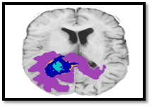
In the Figure 9 the blue version represents the probability of the tumour. It has a wide range of CT scans imaging methods and field strengths, which makes it hard to get consistent segmentation. This makes it hard to get the same results every time. To improve the model's performance and durability, more research needs to be done. Because we broke things down, we came in ninth place overall. As a result, it's hard to figure out which part is most important for improving performance. Post-processing is an option because removing a vessel could have a big impact on our method's final score, so we might want to do that. To avoid overfitting with such a small dataset, and to account for the fact that many variables aren't included in this dataset, we used a multivariate linear regression model.

9.png

Figure 9. Identification of brain tumour after applying the segmentation algorithm

Table 4. Dice and Hausdrff95

To avoid overfitting, our analysis only looked at the volume and surface area of subregions. Many studies have shown that volumetric variables have a big impact on how long people live. These features also make it easier for people who work with patients to use them because they are so common. However, this was not the case in the challenge. More characteristics and expressiveness in models [36] might make it easier to predict how long people will live. It might be better to add clinical information, like molecular and genetic types, to the algorithm in order to improve its accuracy. When we were trying to figure out how to separate brain tumours, we used a group of three-dimensional U-Nets instead of just one model.

5.2 Survival prediction of the results

In the current model, an MRI segmentation data had used to make the survival prediction method. This data came from previously defined parts of the brain tumour. In both the validation and test sets, the model correctly predicted how many patients would live. The IPP was used to figure out how many people survived the whole time. Long-term survivors who have been alive for more than 15 months, short-term survivors (10 months), and mid-term survivors (10-15 months) were all grouped together (in days). Our classifier achieved second out of 60 teams in the test phase. Table 4 shows the results of our method's tests. Because of how the other classifiers works. The Hausdorff Distance (HD) is a regularly used statistic for assessing the performance of various image segmentation methods in the medical industry. On the other hand, present segmentation algorithms do not specifically seek to minimise down on HD. To limit the quantity of HD, we applied U-Net+Logistic three parameters + U-Net+SVM segmentation approaches in this study. In our study three ways are used to construct HD using a probability map built by a U-Net+Logistic three parameters + U-Net+SVM segmentation. According to our findings, the recommended loss functions may lower HD by 18-45 percent while still retaining other segmentation performance measures like the Dice similarity coefficient in perfect working condition. The recommended loss functions can be used to train systems for segmenting medical images so that they don't make major mistakes when they do so.

5.3 Future improvements of the experimental results

In current part, brain tumours are so complicated, it's tough to get exact and trustworthy information about them from MRI scans of them. Improved brain tumour segmentation will need a new technique that looks at brain malignancies in a different way. Both the tumour’s size and how it effects how heated the brain is will be looked at in this session. The thermal profile of the tumour must be broken down next in order to figure out where the tumour boundaries. Because all MRI-based methodologies for temperature mapping need a baseline data set, this study can be extremely beneficial in generating a unique MRI thermal imaging sequence for future studies that look at the absolute temperature distribution.