Aymen Saad* | Javed Ahmed | Ahmed Elaraby
© 2022 IIETA. This article is published by IIETA and is licensed under the CC BY 4.0 license (http://creativecommons.org/licenses/by/4.0/).
OPEN ACCESS
Birds are a reflection of environmental health as pollution and climate change affect bio- diversity. Experts in ecology and machine learning stand to benefit the most from large-scale monitoring of biodiversity. Today, convolutional neural networks (CNNs) are the preferred choice for species recognition as their performance has consistently outperformed humans. However, CNNs are disadvantaged by their high computational complexity and the need to provide vast amounts of training data. This paper compares the performance versus the complexity of two widely used CNNs, namely ResNet- 50 and MobileNetV1. ResNet-50 is a high-complexity CNN while MobilenetV1 is a low-complexity CNN targeted for mobile applications. We used spectrogram images of Brazilian bird sounds as inputs to both networks. These birds were chosen due to their abundance of samples in the Xeno-canto bird sound repository. Short-Time Fourier Transform (STFT) and Mel Frequency Cepstral Coefficient (MFCC) algorithms are used to extracting spectrogram images. To validate the precision of the classifier, 1,000 spectrogram images of each of ten bird species are produced and fed into both classifiers. The findings indicate that the accuracy of MobileNetV1 is close to that of ResNet-50, with MFCC which is 85.73 and 90.56 respectively.
convolutional neural network, spectrogram, bird sound classification, res net, mobile net
Birds are particularly useful ecological markers as they reflect changes in their environment. Studies on the diversity of birds are therefore indispensable [1]. Autonomous recorders are used in bioacoustics monitoring to collect large amounts of audio data from fauna vocalisations [2]. Domain experts can manually identify birds but with larger volumes of information, the process is tedious and time-consuming. Hence a more realistic approach is through machine learning [3-6]. Several bird identifications challenges such as BirdCLEF [2, 7, 8] have been held to evaluate bird sound classifiers. From 2016 onwards, convolutional neural networks (CNNs) have consistently outperformed other classifiers in classifying bird sounds in BirdCLEF [7].
CNN architectures such as Inception-v3 [9] and ResNet [10] perform classification tasks based on the ability of the deep layers of neural network models to extract high-level features from the input images. They are benchmarked using the 1000-image ImageNet dataset [11]. CNNs classify by first converting bird sounds to spectrogram images. However, CNNs are noted for their high computational complexity thus making them unsuitable for applications where the power budgets are restricted. Hence, simpler architectures are continuously being explored to cater to applications where excess accuracy is not required.
The ResNet-50 architecture is a typical state-of-the-art CNN with a depth of 50 layers, 25.6 million arithmetic operations and parameter size of 96 MB [11]. In contrast, the MobileNetV1 has 28 layers deep, requiring 4.2 million operations and a parameter size of 16.9 MB [12].
It is an evolution of the earlier MobileNet targeted for embedded applications [13]. With the simplicity comes to a slight loss in accuracy which is investigated in this paper. Since the performance of both architectures has been measured by ImageNet, they can both classify images into up to 1000 object categories.
CNNs need vast amounts of data to train their network parameters. For bird sounds, training data is plentiful for the more common species. For rarer species, data augmentation is regularly performed to create synthetic samples. In our experiments, both networks were fed with 10,000 sound samples of Brazilian birds. These birds were selected due to the abundance of samples from the Xeno-Canto repository. Each audio clip is resampled and segmented into 1-second samples data at 16 kHz. Each sample containing the bird call signal is then expanded into three samples. Using Short-Time Fourier Transform (STFT) and Mel Frequency Cepstral Coefficient (MFCC) algorithms, the spectrogram representation of the samples is obtained, and then all images are resized using MATLAB 2019b to 224*224. We hypothesize that MobileNetV1 will achieve near ResNet-50 classification accuracy while benefitting from significantly lower computational costs based on the disparity in the number of arithmetic operations of both CNN models.
The CNN-based bird call classifiers are implemented using the methods mentioned below.
2.1 Data preparation
The availability of training data is one of the challenges in employing CNNs. Sound files are readily available for the more common species. For rarer species, data augmentation is regularly performed to create synthetic samples. To address this issue, we used sounds of Brazilian birds as they are abundant in the Xeno-canto sound repository.
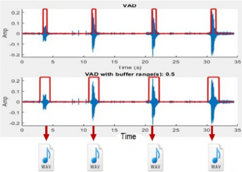
The training dataset for 10 bird species consists of audio files downloaded from the Xeno-canto website, which are then resampled to 16 kHz. Since the training process requires more samples than directly available, the downloaded samples are augmented by segmenting each audio file into several 1 second sound clip files using voice activity detection (VAD) as shown in Figure 1 [14] with 1000 samples are taken for each type of bird selected.
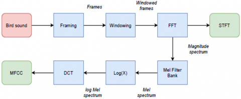
After segmentation, each sound clip is converted into spectrogram images representing the frequency content of the audio in colours. Two algorithms, Short-Time Fourier Transform (STFT) [15] and Mel Frequency Cepstral Coefficients (MFCC) [16] are used to convert sound to image. STFT is applied to the audio signal by splitting the signal into separate overlapping frames, and then computing the Discrete-Time Fourier Transform.
(DTFT) for each frame, resulting in a matrix with complex values as shown in Eq. (1),
$\operatorname{STFT}\{X\}(m, \omega)=X m(\omega)=\sum_{n=-\infty}^{\infty} x_{n} \omega(n-m R) e^{-j \omega n}$ (1)
where, Xn is the input signal at time n, the ω(n) is a Hann window with length m=1024 centred on n, and R = 256 is the hop size between successive frames. The Hann window of size 1024 has a 75% overlap. Once STFT is computed, it can be used to compute MFCC as in Eq. (2):
$\operatorname{Mel}(f)=2595 \log 10\left(1+\frac{f}{700}\right)$ (2)
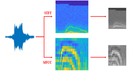
where, m is the Mel scale of the normal frequency scale f. Then, the spectrograms were resized from the original dimension to 224*224*1 to match the input sizes of ResNet50 and MobileNetV1 as shown in Figures 2 and 3 as the 3D image has the highest size compared to the grayscale images. Therefore, 1,000 samples will be prepared to train our proposed classifier for every ten types of bird species.
Figure 1. Voice Activity Detection (VAD) for framing bird vocalizations
Figure 2. Stages in generating STFT and MFCC images
Figure 3. Graphical representation raw audio converted to spectrogram images using STFT and MFCC
2.2 Training setup
The proposed classifier is implemented in MATLAB as follows: the training setup for the 10,000 data samples is done using MATLAB tools.
2.3 Transfer learning
Transfer learning is applied in the proposed classifier to improve learning efficiency in the CNN model. In transfer learning, information that has been previously learned while solving a problem is transferred and reused to solve another related problem [17]. To perform transfer learning, we need to create two components:
These two components were provided as the inputs to the train network function that returns the trained network as an output.
The methodology can descripted as;after completing all the data processing steps, the proposed classifier is built using the MobileNet-v1 architectures. The same classifier is also built using the ResNet50 for validation purposes.
First, the important libraries are prepared, such as Deep Learning Toolbox, Statistics, and Machine Learning Toolbox. These libraries were loaded through the Add-Ons window and then installed on the MATLAB 2019b in order for the code to properly work. The important thing here is using a CUDA-capable NVIDIA GPU with compute capability 3.0, or higher is highly recommended for running this code, where the use of a GPU requires the Parallel Computing Toolbox. Second, Calling the data, the dataset is loaded using an Image Datastore as a data manager. Since Image Datastore operates on image file locations, images are not loaded into memory until reading, making it efficient for the usage of large image collections. Second, we use the imds variable. Third, load images, the classifier contains the images and the category labels associated with each image. The labels are automatically assigned from the folder names of the image. Fourth, Checking the data, in this part, countEachLabel function is used to check and summarize the number of images per category, because the number of images in each class file is unknown. Fifth, Load pre-trained Network, CNN has several pre-trained networks that have gained popularity. Most of these have been trained on the ImageNet dataset, which has 1000 object categories and 1.2 million training images. ResNet50 and MobileNetv1 are such models that could be loaded using the function from Neural Network Toolbox. Sixth, Prepare the data, Preparation of training and testing image datasets involves splitting the sets into training and validation data. As a common practice, 80% of images from each set are chosen randomly for the training data and the remainder, 20%, for the validation (testing) data. Randomization is important during the split to avoid biasing results. Seventh, Reduce output, The CNN architectures are suitable for large-scale classification of up to 1000 species due to the deep layer of neural network models to obtain high-level feature extraction from the spectrogram image. However, the proposed classifier system is targeting low complexity devices. Therefore, the 1000 layers are reduced to 10 layers.
This section discusses the validation results of our low complexity CNN model, MobileNetV1, where the accuracy is benchmarked with the high complexity model, ResNet-50.
3.1 Training stage outcome
In the proposed classifier, there are 8,000 images extracted from the training dataset, where each bird species derives 800 spectrogram images. These images were processed in the training stage of two CNN models:
In both CNN models, five epochs are applied, which means that each type of dataset is processed in the training stage five times. Thus, we have 6665 iterations and 1333 iterations per epoch. The details of the results are shown in Table 2.
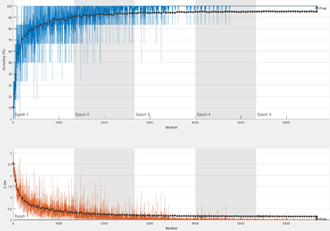
Figure 4. Training accuracy
Table 1. Six-letter alpha codes for birds in the study
|
No |
English Name |
Scientific Name |
Six-letter Alpha Codes |
|
1 |
Eurasian Wigeon |
Mareca penelope |
MARPEN |
|
2 |
American Robin |
Turdus migratorius |
TURMIG |
|
3 |
Eurasian Skylark |
Alauda arvensis |
ALAARV |
|
4 |
Purple Honeycreeper |
Cyanerpes caeruleus |
CYACAE |
|
5 |
White-winged Dove |
Zenaida asiatica |
ZENASI |
|
6 |
Brown Shrike |
Lanius cristatus |
LANCRI |
|
7 |
Northern Lapwing |
Vanellus vanellus |
VANVAN |
|
8 |
Long-billed Hermit |
Phaethornis longirostris |
PHALON |
|
9 |
Pigeon Guillemot |
Cepphus columba |
CEPCOL |
|
10 |
Swallow Tanager |
Tersina viridis |
TERVIR |
Accuracy and loss are observed through the training progress as shown in Figure 4. The accuracy increases as the epoch increase until it reaches a saturated level, where inaccuracy is very small and it fluctuates at a certain level. It is decaying, but the loss decreases as the epoch decreases until it reaches a certain saturation level. In other words, accuracy determines how good the model is, and loss determines how bad the model is. A good model usually comes with high accuracy and low loss.
3.2 Testing stage (validation) outcome
The testing or validation dataset is a dataset that is independent of the training dataset, but that follows the same probability distribution as the training dataset. In the proposed classifier, there are 2,000 images of ten bird species, where each bird species has 200 images. Table 1 lists the (English Name, Scientific Name and Six-letter Alpha Codes) for all the ten birds [18].
A confusion matrix shows how well the model can accurately predict the class that is used in supervised learning. In the validation test of the proposed model, the model predicts the respective classes of the ten species. Each column of the matrix represents the number of predictions of each class, while each row represents the instances in the real class. The outputs are recorded in the confusion matrix. The highlighted area is the number of correctly predicted output. It presents the prediction by using the colour hue. For example, for the class with high accuracy which is between 90-100%, the block has a dark colour, but when the model is slightly confused between two or more classes and cause the accuracy drop to between 80-89%, the block has a lighter colour. The much lighter block is applied when the model is quite confused and cause the accuracy to drop between 60-79%, and so on.
The first confusion matrix, as shown in Table 2 is for the high complexity model, ResNet-50 with STFT feature extraction. It is clearly showing that there are several significantly dark blocks such as classes 1, 3, 4, 6, 7, 8, and 9 since the accuracy is above 90%, which is very high. A slightly lighter shade is applied to blocks with accuracy between 80-89% such as classes 2 and 5. Another class, which is class 10 is in the much lighter shade since it has the lowest accuracy, which is 68%. The blocks which are the confused classes have quite a lighter shade rather than the correct classes in the diagonal line.
The second confusion matrix, as in Table 3 is for the ResNet-50 model with MFCC feature extraction. The significantly dark blocks have high accuracy such as classes 3, 4, 7, 8, and 10, which are above 90%. The lighter shade blocks such as classes 1 and 9 have an accuracy between 80-89%, while classes 2 and 6 are in the much lighter shade with the lowest accuracy of 59%. The confused blocks are rather lighter than the correct blocks in the diagonal, which is less than 30% of accuracy.
Table 2. Confusion matrix for ResNet-50 with STFT
|
1 |
94.1 |
0.5 |
0 |
2.5 |
2.5 |
0 |
2 |
0.5 |
0 |
3.3 |
|
2 |
2.2 |
87.2 |
0 |
1 |
6.1 |
0.6 |
0.5 |
0.5 |
1.7 |
4.1 |
|
3 |
0 |
0 |
97.1 |
0 |
0 |
0 |
0 |
0 |
0 |
0 |
|
4 |
0 |
0 |
0 |
93.6 |
2 |
0 |
0 |
0.5 |
0 |
0.8 |
|
5 |
0 |
0 |
0 |
0.5 |
81.1 |
0 |
0 |
0 |
0 |
0.4 |
|
6 |
1.1 |
1.6 |
0.5 |
1 |
4.9 |
94.2 |
0 |
0 |
2.8 |
12.4 |
|
7 |
0 |
0 |
0 |
1 |
0.8 |
0 |
96 |
0 |
0 |
0.8 |
|
8 |
0 |
0.5 |
0 |
0 |
0 |
0 |
0.5 |
98 |
0 |
0 |
|
9 |
0 |
5.9 |
0 |
0 |
0.8 |
1.3 |
0 |
0.5 |
92 |
9.1 |
|
10 |
1.6 |
3.7 |
2.4 |
0.5 |
1.6 |
3.9 |
1 |
0 |
3.4 |
68.9 |
|
1 |
2 |
3 |
4 |
5 |
6 |
7 |
8 |
9 |
10 |
Table 3. Confusion matrix for ResNet-50 with MFCC
|
1 |
91.3 |
3.9 |
0 |
0 |
0 |
1.4 |
1.7 |
0 |
0 |
1 |
|
2 |
0 |
49.7 |
0 |
0 |
1.1 |
1 |
0 |
0 |
1.8 |
0 |
|
3 |
0 |
0 |
99.5 |
0 |
0 |
1.4 |
0 |
0 |
0 |
0 |
|
4 |
1 |
3.1 |
0 |
98.9 |
1.1 |
1 |
0 |
0 |
0 |
0 |
|
5 |
0 |
4.9 |
0 |
0 |
95.8 |
0 |
0 |
0 |
0 |
0 |
|
6 |
1 |
4.9 |
0 |
0.5 |
0 |
83.3 |
0 |
0 |
1.8 |
0 |
|
7 |
1.5 |
6.4 |
0 |
0 |
0.5 |
0 |
97.7 |
0 |
0 |
0 |
|
8 |
2.6 |
2.1 |
0 |
0 |
0 |
0 |
0.6 |
98 |
0 |
0 |
|
9 |
0 |
8 |
0 |
0 |
0.5 |
2.4 |
0 |
0.5 |
94.1 |
2.9 |
|
10 |
2.6 |
17 |
0.5 |
0.5 |
1.1 |
9.5 |
0 |
0 |
2.4 |
96.2 |
|
|
1 |
2 |
3 |
4 |
5 |
6 |
7 |
8 |
9 |
10 |
Table 4. Confusion matrix for MobileNetV1 with STFT
|
1 |
64.3 |
3.9 |
0.9 |
1.6 |
0 |
0 |
2.5 |
1.3 |
3.4 |
4.1 |
|
2 |
2.9 |
48.9 |
2.3 |
2.6 |
0 |
0 |
1.3 |
2.2 |
1 |
5.4 |
|
3 |
2 |
0.3 |
85.5 |
1.6 |
0 |
0 |
0.6 |
0.9 |
1 |
0 |
|
4 |
2 |
0.6 |
0.5 |
61.7 |
0 |
0 |
0 |
0 |
0 |
1.4 |
|
5 |
2 |
9.4 |
4.2 |
15.9 |
92.3 |
0 |
11.9 |
2.6 |
3.7 |
6.8 |
|
6 |
12.3 |
13.3 |
1.4 |
4.5 |
1.5 |
100 |
3.8 |
3.1 |
18.9 |
21.6 |
|
7 |
3.3 |
8.8 |
2.3 |
7.5 |
1.5 |
0 |
70.4 |
1.3 |
4.4 |
4.1 |
|
8 |
0.4 |
1.2 |
0 |
0.3 |
0 |
0 |
0.6 |
82.8 |
1 |
1.4 |
|
9 |
3.7 |
4.5 |
0.5 |
1.3 |
1.5 |
0 |
0.6 |
2.2 |
54.9 |
0.7 |
|
10 |
7 |
9.1 |
2.3 |
2.9 |
3.1 |
0 |
8.2 |
3.5 |
11.8 |
54.7 |
|
|
1 |
2 |
3 |
4 |
5 |
6 |
7 |
8 |
9 |
10 |
Table 5. Confusion matrix for ResNet-50 with MFCC
|
1 |
81.3 |
3.9 |
0 |
0.5 |
0.9 |
2.9 |
0 |
0 |
1 |
0 |
|
2 |
1.4 |
59.2 |
0 |
0.5 |
3.2 |
0.6 |
0 |
0.5 |
1.5 |
0 |
|
3 |
0 |
0.3 |
95.7 |
0 |
0 |
0 |
0.7 |
0 |
0 |
0 |
|
4 |
1.4 |
0.3 |
0 |
95.6 |
0 |
0 |
0 |
0 |
0 |
0 |
|
5 |
1.9 |
1.3 |
1 |
0 |
84.4 |
1 |
0 |
0 |
1.5 |
0 |
|
6 |
0.9 |
1.9 |
0.5 |
0 |
0.5 |
59.7 |
0 |
0 |
3 |
0 |
|
7 |
2.3 |
6.5 |
1.4 |
2.4 |
5 |
5.8 |
99.3 |
0 |
1 |
0 |
|
8 |
0.9 |
4.2 |
0 |
0 |
0 |
0 |
0 |
98.9 |
0.5 |
0 |
|
9 |
1.4 |
4.9 |
0 |
0.5 |
1.4 |
4.5 |
0 |
0 |
82.8 |
0 |
|
10 |
8.4 |
17.5 |
1.4 |
0.5 |
4.6 |
25.3 |
0 |
0.5 |
8.6 |
100 |
|
|
1 |
2 |
3 |
4 |
5 |
6 |
7 |
8 |
9 |
10 |
On the other hand, Table 4 shows the confusion matrix for MobileNetV1 with STFT feature extraction. In this case, there are only two blocks with a significantly dark shade, which are classes 5 and 6, where class 5 is 92.3%, and class 6 is perfectly 100%. The blocks with lighter shades are classes 3 and 8 with an accuracy between 80-89%, and the other classes have grey shades.
Lastly, Table 5 shows the confusion matrix MobileNetV1 with MFCC feature extraction. In this case, we can see some classes have the darker blocks that mean high accuracy, which is above 90% such as 3, 4, 7 and 10, but the lighter blocks such as 1 and 9 classes have the accuracy between (80-89) %, and the other classes have the much lighter colour. The confused block in both low complexity models is seen as greater than the high complexity model, but they are still under the 30% accuracy.
3.3 Summary of results
Accuracy is a quality measurement of the proposed model, which also translate into how well it could make a new prediction based on the data it has never seen before. The time is how long the testing progress will take to be finished. Table 6 illustrates the accuracy and time to load the trained model and response time after recording.
The accuracy is calculated using the formula as follows:
Accuracy $=\frac{\text { Number of correct predictions }}{\text { Total predictions }}$ (3)
From Table 6, the high complexity model, which is ResNet-50, is observed to have higher accuracy, but requires a longer time to make a prediction, compared to the low complexity model. This is due to a large number of operations, which is 25.6 million. The high complexity model is also bigger at 96 MB. On the other hand, the low complexity model, which is MobileNetV2 has a smaller number of operations that results in a shorter testing time. Besides, it is also smaller in size, but we can observe that it has slightly lower accuracy. This result comes as expected, where a high complexity model would advantage more on the accuracy, but suffers in terms of size and time. In contrast, the low complexity model has sufficient accuracy without need to compromise the model size and testing time.
To be more specific the performance measures used in this study (see Tables 7-10) are the most widely used metrics shown below in Eqns. (4), (5), (6) and (7) are sensitivity, specificity, accuracy, and precision [19] which are given as:
Sensitivity $=\frac{T P}{T P+F N}$ (4)
Specificity $=\frac{T N}{T N+F P}$ (5)
Precision $=\frac{T P}{T P+F P}$ (6)
F_Measure $=\frac{2 * T P}{2 * T P+F P+F N}$ (7)
Table 6. Summary of results
|
Type of model |
#Operations [million] |
Size [MB] |
Time (min) |
Accuracy |
|
ResNet-50 (STFT) |
25.6 |
96 |
941 |
90.40 |
|
ResNet-50 (MFCC) |
523 |
90.56 |
||
|
MobileNet-v1 (STFT) |
4.2 |
16.9 |
160 |
71.57 |
|
MobileNet-v1 (MFCC) |
187 |
85.73 |
Table 7. Evaluation metrics result using ResNet-50 (STFT)
|
NAME OF CLASS |
Ac. |
Sen. |
Spe. |
Pre. |
F-measure |
|
MARPEN |
0.98 |
0.89 |
0.99 |
0.95 |
0.92 |
|
TURMIG |
0.97 |
0.84 |
0.99 |
0.88 |
0.86 |
|
ALAARV |
1.00 |
1.00 |
1.00 |
0.97 |
0.99 |
|
CYACAE |
0.99 |
0.97 |
0.99 |
0.94 |
0.95 |
|
ZENASI |
0.98 |
0.99 |
0.98 |
0.81 |
0.89 |
|
LANCRI |
0.97 |
0.97 |
1.00 |
0.94 |
0.86 |
|
VANVAN |
0.99 |
97 |
1.00 |
0.96 |
0.97 |
|
PHALON |
1.00 |
0.99 |
1.00 |
0.98 |
0.98 |
|
COLUOE |
0.97 |
0.84 |
0.99 |
0.92 |
0.88 |
|
TERPVI |
0.95 |
0.79 |
0.96 |
0.69 |
0.74 |
Table 8. Result of all evaluation metrics usingResNet-50 (MFCC)
|
NAME OF CLASS |
Ac. |
Sen. |
Spe. |
Pre. |
F-measure |
|
MARPEN |
0.98 |
0.99 |
0.94 |
0.50 |
0.92 |
|
TURMIG |
0.94 |
0.93 |
0.65 |
0.50 |
0.65 |
|
ALAARV |
1.00 |
0.99 |
1.00 |
1.00 |
0.99 |
|
CYACAE |
0.99 |
0.94 |
1.00 |
0.99 |
0.96 |
|
ZENASI |
0.99 |
0.95 |
0.99 |
0.96 |
0.95 |
|
LANCRI |
0.97 |
0.91 |
0.98 |
0.83 |
0.87 |
|
VANVAN |
0.99 |
0.92 |
1.00 |
0.98 |
0.95 |
|
PHALON |
0.99 |
0.95 |
1.00 |
0.99 |
0.97 |
|
COLUOE |
0.98 |
0.87 |
0.99 |
0.94 |
0.90 |
|
TERPVI |
0.96 |
0.74 |
0.99 |
0.94 |
0.84 |
Table 9. Result of all evaluation metrics by using MobileNet-v1 (STFT)
|
NAME OF CLASS |
Ac. |
Sen. |
Spe. |
Pre. |
F-measure |
|
MARPEN |
0.98 |
0.85 |
0.99 |
0.93 |
0.89 |
|
TURMIG |
0.96 |
0.75 |
0.98 |
0.80 |
0.98 |
|
ALAARV |
1.00 |
1.00 |
1.00 |
0.97 |
0.89 |
|
CYACAE |
0.99 |
0.95 |
0.99 |
0.90 |
0.93 |
|
ZENASI |
0.94 |
0.79 |
0.97 |
0.83 |
0.81 |
|
LANCRI |
0.99 |
0.99 |
0.99 |
0.95 |
0.97 |
|
VANVAN |
0.99 |
0.96 |
0.99 |
0.95 |
0.96 |
|
PHALON |
1.00 |
0.99 |
1.00 |
0.97 |
0.98 |
|
COLUOE |
0.97 |
0.76 |
0.99 |
0.87 |
0.81 |
|
TERPVI |
0.94 |
0.75 |
0.96 |
0.64 |
0.54 |
Table 10. Result of all evaluation metrics by using MobileNet-v1 (MFCC)
|
NAME OF CLASS |
Ac. |
Sen. |
Spe. |
Pre. |
F-measure |
|
MARPEN |
0.98 |
0.88 |
0.99 |
0.94 |
0.91 |
|
TURMIG |
0.97 |
0.78 |
0.98 |
0.83 |
0.80 |
|
ALAARV |
1.00 |
1.00 |
1.00 |
0.97 |
0.99 |
|
CYACAE |
99 |
0.97 |
0.99 |
0.94 |
0.95 |
|
ZENASI |
0.95 |
0.78 |
0.98 |
0.82 |
0.80 |
|
LANCRI |
0.99 |
0.99 |
0.99 |
0.91 |
0.95 |
|
VANVAN |
0.99 |
0.97 |
0.99 |
0.96 |
0.97 |
|
PHALON |
1.00 |
0.99 |
1.00 |
0.98 |
0.98 |
|
COLUOE |
0.97 |
0.82 |
0.99 |
0.91 |
0.87 |
|
TERPVI |
0.95 |
0.85 |
0.96 |
0.76 |
0.80 |
True Positive (TP): Number of correctly labelled positive samples. False Positive (FP): Number of negative samples incorrectly labelled as positive. True Negative (TN): Number of correctly labelled negative samples. False Negative (FN): Number of positive samples incorrectly labelled as negative.
Low complexity CNN-based bird call classifier is proposed where the MobileNetV1 model is employed. Audio samples of ten bird species from the Xeno-Canto website are used as the dataset. Each audio sample is spliced into short 1-second clips and the noise is removed using VAD. Besides, augmentation of the short clips is performed to vary the samples up to 1,000 sound clips per species. Then, the sound clips are converted into spectrogram images using STFT and MFCC conversion for feature extraction and resized to 224 224 to fit the CNN input. The output layer is also modified into ten layers. Finally, the work is benchmarked with a high-complexity CNN model, ResNet-50. From the results, the proposed classifier has sufficient accuracy without need to compromise the model size and testing time.
[1] Priyadarshani, N., Marsland, S., Castro, I. (2018). Automated birdsong recognition in complex acoustic environments: A review. Journal of Avian Biology, 49(5): jav-01447. https://doi.org/10.1111/jav.01447
[2] Kahl, S., Stöter, F.R., Goëau, H., Glotin, H., Planque, R., Vellinga, W.P., Joly, A. (2019). Overview of BirdCLEF 2019: Large-scale bird recognition in soundscapes. In Working Notes of CLEF 2019-Conference and Labs of the Evaluation Forum, 2380: 1-9. https://hal.umontpellier.fr/hal-02345644
[3] Towsey, M., Planitz, B., Nantes, A., Wimmer, J., Roe, P. (2012). A toolbox for animal call recognition. Bioacoustics, 21(2): 107-125. https://doi.org/10.1080/09524622.2011.648753
[4] Cai, J., Ee, D., Pham, B., Roe, P., Zhang, J. (2007). Sensor network for the monitoring of ecosystem: Bird species recognition. In 2007 3rd International Conference on Intelligent Sensors, Sensor Networks and Information, pp. 293-298. https://doi.org/10.1109/ISSNIP.2007.4496859
[5] Trifa, V.M., Kirschel, A.N., Taylor, C.E., Vallejo, E.E. (2008). Automated species recognition of antbirds in a Mexican rainforest using hidden Markov models. The Journal of the Acoustical Society of America, 123(4): 2424-2431. https://doi.org/10.1121/1.2839017
[6] Briggs, F., Lakshminarayanan, B., Neal, L., Fern, X.Z., Raich, R., Hadley, S.J., Betts, M.G. (2012). Acoustic classification of multiple simultaneous bird species: A multi-instance multi-label approach. The Journal of the Acoustical Society of America, 131(6): 4640-4650. https://doi.org/10.1121/1.4707424
[7] Goëau, H., Glotin, H., Vellinga, W.P., Planqué, R., Joly, A. (2016). Lifeclef bird identification task 2016: The arrival of deep learning. In CLEF: Conference and Labs of the Evaluation Forum, 1609: 440-449. https://hal.archives-ouvertes.fr/hal-01373779
[8] Lasseck, M. (2019). Bird species identification in soundscapes. In CLEF (Working Notes), 2380.
[9] Bai, J., Wang, B., Chen, C., Chen, J., Fu, Z. (2019). Inception-v3 Based Method of LifeCLEF 2019 Bird Recognition. In CLEF (Working Notes).
[10] Sankupellay, M., Konovalov, D. (2018). Bird call recognition using deep convolutional neural network, ResNet-50. In Proceedings of ACOUSTICS, 7(9): 1-8.
[11] Russakovsky, O., Deng, J., Su, H., Krause, J., Satheesh, S., Ma, S., Fei-Fei, L. (2015). Imagenet large scale visual recognition challenge. International Journal of Computer Vision, 115(3): 211-252. https://doi.org/10.1007/s11263-015-0816-y
[12] Kahl, S., Wilhelm-Stein, T., Klinck, H., Kowerko, D., Eibl, M. (2018). Recognizing birds from sound-the 2018 BirdCLEF baseline system. arXiv preprint arXiv:1804.07177.
[13] Howard, A.G., Zhu, M., Chen, B., Kalenichenko, D., Wang, W., Weyand, T., Adam, H. (2017). Mobilenets: Efficient convolutional neural networks for mobile vision applications. arXiv preprint arXiv:1704.04861.
[14] Moattar, M.H., Homayounpour, M.M. (2009). A simple but efficient real-time voice activity detection algorithm. In 2009 17th European Signal Processing Conference, pp. 2549-2553.
[15] Baba, T. (2012). Time-frequency analysis using short time Fourier transform. The Open Acoustics Journal, 5(1): 32-38. https://doi.org/10.2174/1874837601205010032
[16] Lee, C.H., Han, C.C., Chuang, C.C. (2008). Automatic classification of bird species from their sounds using two-dimensional cepstral coefficients. IEEE Transactions on Audio, Speech, and Language Processing, 16(8): 1541-1550. https://doi.org/10.1109/TASL.2008.2005345
[17] Fritzler, A., Koitka, S., Friedrich, C.M. (2017). Recognizing Bird Species in Audio Files Using Transfer Learning. In CLEF (Working Notes).
[18] Pyle, P., DeSante, D.F. (2015). Four-letter (English name) and six-letter (scientific name) alpha codes for 2116 bird species (and 98 non-species taxa) in accordance with the 56th AOU Supplement (2015).
[19] Baratloo, A., Hosseini, M., Negida, A., El Ashal, G. (2015). Part 1: Simple definition and calculation of accuracy, sensitivity and specificity. Emergency (Tehran, Iran), 3(2): 48-49. https://doi.org/10.22037/emergency.v3i2.8154