Dianru Jia* | Jianju Yang
© 2022 IIETA. This article is published by IIETA and is licensed under the CC BY 4.0 license (http://creativecommons.org/licenses/by/4.0/).
OPEN ACCESS
There is a huge demand for high-quality images, whether in human visual perception or image applications. The existing methods for image enhancement ignore the influence of incident light on real color images. As a result, the output images are often not effectively enhanced or not natural, and the enhancement effect is not ideal for multi-scale images. To solve the problem, this paper presents a multi-scale image enhancement algorithm based on deep learning and illumination compensation. Firstly, a compensation algorithm was developed for image illumination drift based on the Hodge decomposition model. Then, low-illumination multi-scale images were enhanced by a lightweight multi-scale Retinex network, and the architecture of that network was explained in details. After that, a new joint network loss function was designed for the input and output forms, corresponding to the proposed deep learning network, and the low-illumination multi-scale image enhancement. Experimental results demonstrate that the proposed model can effectively enhance multi-scale images.
deep learning, illumination compensation, multi-scale image enhancement
Image is the main carrier and primary way of expression for visual information [1-9]. When the illumination is insufficient or ununiform, or blocked by objects, the captured images often have visual problems like as low brightness, high noise, and low contrast [10-17]. High-quality images are always expected, whether in human visual perception or in image applications [18-25]. If a dark low-illumination image, which does not conform to the visual perception of the human eyes, can be easily converted into a normal light image, it would bring great convenience to our daily life.
Low or uneven brightness reduces the contrast of near-infrared and optical remote sensing images, making it challenging to analyze the image contents. Huang et al. [26] proposed a spatially adaptive method to enhance multi-scale images: the nonsubsampled contourlet transform is adopted to decompose each low-contrast image into multiple scales; based on improved histogram equalization, a spatially adaptive gamma correction strategy is presented to enhance the base layer, which serves as the guide layer. Zhou et al. [27] applied the style transfer of CycleGAN (generative adversarial network) to low-illumination image enhancement. During the network structural design, different convolution kernels were used to extract features from three paths, and a deep residual shrinkage network was developed to suppress the noise after convolution. Both visual effects and objective indices show that the CycleGAN, which is based on multi-scale deep residual shrinkage, performs excellently in low-illumination enhancement, detail restoration, and denoising. Zhou et al. [28] proposed a multi-scale Retinex-based adaptive grayscale transform approach for underwater image enhancement. Their approach consists of three steps: color correction, image denoising, and detail enhancement. For different degraded underwater images, simulated annealing optimization was introduced to implement adaptive grayscale transform, and enhance image details. Pan et al. [29] created a multi-scale fusion residual encoder-decoder approach for low-illumination image enhancement. The approach directly learns the end-to-end mapping between the original light and dark images from the original sensor, and fully restores the details and colors of the original image, while effectively enhancing the image brightness. To improve the quality of image textures, Yuan et al. [30] put forward a multi-scale fusion enhancement method. Two new fusion inputs were obtained by different color methods. One input was utilized in the red-green-blue (RGB) model to improve image resolution before de-stacking, through the contrast-based dark channel. The other input was adopted for color compensation, based on multiple morphological operations and the opponent colors in the CIE 1976 L*a*b* color model.
The existing methods need to be improved in terms of detail processing and noise reduction. None of them fully consider the effects of nonuniform light intensity. Besides, these methods ignore the influence of incident light on real color images. As a result, the output images are often not effectively enhanced or not natural, and the enhancement effect is not ideal for multi-scale images. To solve the problem, this paper presents a multi-scale image enhancement algorithm based on deep learning and illumination compensation. Section 2 develops a compensation algorithm for image illumination drift based on the Hodge decomposition model. Section 3 enhances low-illumination multi-scale images by a lightweight multi-scale Retinex network, details the architecture of that network, and designs a new joint network loss function for the input and output forms, corresponding to the proposed deep learning network, and the low-illumination multi-scale image enhancement. Experimental results demonstrate the effectiveness of the proposed model.
For the same image, the uneven illumination in different areas is often related to the optical path design for imaging. This problem can be solved by properly designing the optical paths. However, the optical path design needs to modify the hardware, and cannot overcome illumination drift. Based on the Hodge decomposition model, this paper compensates for the illumination of the image to be enhanced. This approach can effectively solve the uneven illumination within or strong illumination drift of the image.
In this paper, the image decomposition model is introduced into a simplified form of Hodge decomposition, which realizes the decomposition of the low-frequency harmonic function and the high-frequency random disturbance term, that is, the decomposition of the smooth illumination component and the high-frequency texture component.
For a given image g(a0,b0), the Hodge decomposition can be defined as:
$g\left( {{a}_{0}},{{b}_{0}} \right)=v\left( {{a}_{0}},{{b}_{0}} \right)+u\left( {{a}_{0}},{{b}_{0}} \right),\forall \left( {{a}_{0}},{{b}_{0}} \right)\in \Omega $ (1)
Pose component v(a0,b0) is a harmonic function, and u(a0,b0) is locally square integrable, with a zero mean. Let φ(a,b|a0,b0) be the low-pass filter. Then, we have:
$\int{\int{_{{{M}_{\phi }}\left( {{a}_{0}},{{b}_{0}} \right)}}}u\left( a,b \right)\phi \left( a,b|{{a}_{0}},{{b}_{0}} \right)dadb=0$ (2)
Let component u(a0,b0) denote the texture of image g(a0,b0). Formula (2) shows that: u(a0,b0) as a texture feature should be a high-frequency signal. Under ideal conditions, the convolution of u(a0,b0) and φ(a,b|a0,b0) is equal to 0. Besides, the assumption that u(a0,b0) is locally square integrable, with a zero mean, can be assured by substituting the following Hodge decomposition formula into formula (2):
$u\left( a,b \right)=g\left( a,b \right)-v\left( a,b \right)$ (3)
Since component u(a0,b0)is square integrable, the variance Ω(u(a0,b0)) can be used to estimate the regression variance for linear drift.
In the field of illumination compensation, a hot topic is the intrinsic image decomposition based on Renitex theory. By the intrinsic image decomposition model, image g(a0,b0) can be decomposed into two components, namely, reflectivity S(a0,b0), and illuminance gain v(a0,b0). The intrinsic image decomposition formula for g(a0,b0) can be expressed as:
$g\left( {{a}_{0}},{{b}_{0}} \right)=S\left( {{a}_{0}},{{b}_{0}} \right)\cdot v\left( {{a}_{0}},{{b}_{0}} \right)$ (4)
If the image has a uniform texture, the reflectivity of its surface is basically constant. According to the Renitex theory, S(a0,b0)=D and ∀(a0,b0)ÎΓ. Thus, g(a0,b0)= D·v(a0,b0).
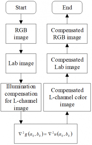
The basic idea of our multi-scale image illumination compensation approach is to replace the illumination component of image Hodge decomposition with a constant, thereby eliminating the influence of illumination changes. Figure 1 shows the flow of the proposed illumination compensation algorithm.
Figure 1. Flow of the proposed illumination compensation algorithm
To realize the Hodge decomposition of a given grayscale image, the first step is to acquire the texture component of the image by solving the partial differential equation. Through Laplacian second-order differential operation on both sides of the equation for the Hodge decomposition of the given image g(a0,b0), we have:
${{\nabla }^{2}}g\left( {{a}_{0}},{{b}_{0}} \right)={{\nabla }^{2}}v\left( {{a}_{0}},{{b}_{0}} \right)+{{\nabla }^{2}}u\left( {{a}_{0}},{{b}_{0}} \right)$ (5)
Considering the harmony of v(a0,b0), i.e., ∇2v(a0,b0) is 0, we have:
${{\nabla }^{2}}g\left( {{a}_{0}},{{b}_{0}} \right)={{\nabla }^{2}}u\left( {{a}_{0}},{{b}_{0}} \right)$ (6)
The texture component of g(a0,b0) can be obtained by solving formula (6). After calculating the component u(a0,b0), the Hodge component v(a0,b0) can be obtained by v(a0,b0)=g(a0,b0)-u(a0,b0). Given the deviation z>0, the illuminance component v(a0,b0) in the Hodge decomposition is replaced by z to obtain the compensated image g*(a0,b0):
${{g}^{*}}\left( {{a}_{0}},{{b}_{0}} \right)=z+u\left( {{a}_{0}},{{b}_{0}} \right)$ (7)
Let PD be the public deviation in the entire database. Then, the Gabor filter response for g*(a0,b0) can be expressed as:
${{G}^{*}}\left( {{a}_{0}},{{b}_{0}},\varepsilon ,\omega \right)=PD+U\left( {{a}_{0}},{{b}_{0}},\varepsilon ,\omega \right)$ (8)
According to the above formula, the Gabor filter response is independent of the illuminance v(a0,b0), i.e., the influence of the illuminance on the image texture feature is eliminated.
If the image is a color image, the illumination compensation needs to first convert the original image from the RGB color space to the Lab color space, before implementing illumination compensation on the grayscale image g(a0,b0) of the L channel in the Lab color space. In this way, it is possible to obtain a compensated L-channel color image g*(a0,b0).
Formula (6) is a second-order elliptic partial differential equation, which can be calculated numerically by the finite difference method. Let matrices Up and Q be the discretization of functions u(a,b) and ∇2g(a,b), respectively. Then, the iterative equation of the finite difference method can be expressed as:
$U_{t,w}^{p+1}=\frac{1}{4}\left( U_{t-1,w}^{p}+U_{t+1,w}^{p}+U_{t,w-1}^{p}+U_{t,w+1}^{p}-{{Q}_{t,w}} \right)$ (9)
Formula (9) can be realized through image filtering. Let matrix G be the discretization of the original multiscale color image g(a,b). Formula (9) can be initialized by:
$U_{t,w}^{0}={{G}_{t,w}}$ (10)
Different form formula (9), the boundary condition of the color image filter should be set to the Neumann boundary condition of formula (6), in order to realize the real algorithm. Let ∂u/∂m be the directional derivative of function u(a,b) along the normal direction of the boundary. We have:
${{\left[ \frac{\partial u}{\partial m} \right]}_{\partial \Omega }}=0$ (11)
If a low-illumination image enhancement algorithm boasts a good enhancement effect and a low time complexity, then the corresponding visual system will perform excellently. Both accuracy and real-timeliness are two key parameters of a good image enhancement algorithm. Otherwise, the algorithm would be unsuitable for wide application. Traditionally, low-illumination image enhancement methods are mostly based on physical models. Despite their good robustness and generalization ability, these methods cannot achieve ideal enhancement effect, when the external illumination is very complex. The deep learning-based image enhancement algorithms can realize the enhancement requirements of the visual system. In multi-scene and low-illumination conditions, the traditional deep learning models have a limited generalization ability, which does not apply to low-illumination images in a complex background. Besides, their algorithms consume too much time, failing to meet the real-time visual needs. Therefore, this paper chooses the lightweight multi-scale Retinex network to enhance low-illumination multi-scale images. The selected network can fully satisfy the actual needs, for its good performance and simple structure.
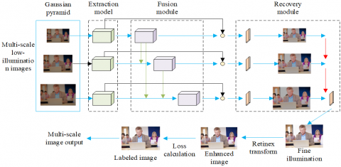
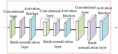
Figure 2 shows the architecture of lightweight multi-scale Retinex network, which encompasses four modules. To mine the image features of multiple scales, the Gaussian pyramid module performs multi-scale decomposition of the low-illumination images. To obtain the initial illumination, the illumination extraction module estimates and extracts the illumination information in multi-scale images. To obtain fused illumination, the illumination fusion module merges the extracted deep features and cross-scale features of multi-scale lights. To get fine illumination, the recovery module integrates and adjusts the fusion of multi-scale lights. Finally, the enhanced multi-scale image is obtained by Retinex transform. Figure 3 presents the multi-layer structure of the illumination extraction module.
Figure 2. Architecture of lightweight multi-scale Retinex network
Figure 3. Structure of the illumination extraction module
The single-scale Retinex algorithm is difficult to determine the scale parameter τ. This limitation can be overcome by the MSR-Net, a deep learning network based on the multi-scale Retinex algorithm. The key processing steps of the network can be expressed as:
$QU\left( a,b \right)=S\left( a,b \right)\times K\left( a,b \right)$ (12)
$s(a, b)=\log (S(a, b))=\log (Q U(a, b))-\log (K(a, b))$ (13)
$s\left( a,b \right)=log\left( QU\left( a,b \right) \right)-log\left( G\left( a,b \right)\otimes QU\left( a,b \right) \right)$ (14)
$s\left( a,b \right)=log\left( QU\left( a,b \right) \right)-{}^{1}/{}_{3}log\left( \sum\limits_{m=1}^{3}{{{L}_{m}}{{o}^{-\frac{{{a}^{2}}+{{b}^{2}}}{2\tau _{m}^{2}}}}}\otimes QU\left( a,b \right) \right)$ (15)
In deep learning models, the loss function guides the network training, exerting a huge impact on the mapping ability of the original input to the actual results. This paper designs a new joint network loss function for the input and output forms, corresponding to the proposed deep learning network, and the low-illumination multi-scale image enhancement. The function involves seven loss terms: trend consistency loss KTC, color consistency loss KCC, local loss KLO, exposure control loss KEC, mean squared error loss function KJF, structural similarity loss function KJG, and smoothing loss function KPH. The weights of the corresponding loss terms in the joint loss function are represented by qs, qx, qn, qrr, and qr, respectively. The joint network loss function can be given by:
$K={{K}_{TC}}+{{K}_{LO}}+{{q}_{s}}{{K}_{EC}}+{{q}_{x}}{{K}_{CC}}+{{q}_{n}}{{K}_{JF}}+{{q}_{rr}}{{K}_{JG}}+{{q}_{r}}{{K}_{PH}}$ (16)
Each loss term is detailed below. Firstly, the trend graph was calculated based on the traditional calculation of image gradient graph. Let ∇cg(a,b) be the first-order gradient a certain direction c of the image g(a,b); f and q be the vertical and horizontal directions of direction c, respectively; p be a random integer. Then, the trend value of g(a,b) in a certain direction can be calculated by:
${{\bar{\nabla }}_{c}}g\left( a,b \right)=\left\{ \begin{align} & p\text{ }\nabla {{g}_{c}}\left( a,b \right)>0 \\ & 0\text{ }\nabla {{g}_{c}}\left( a,b \right)=0 \\ & -p\text{ }\nabla {{g}_{c}}\left( a,b \right)<0 \\\end{align} \right\},c\in \left\{ f,q \right\}$ (17)
Let ∇*Ṙ be the trend graph of the enhanced image Ṙ; ∇*R be the mean of the trend graph of the original image R; ∇*Ṙij be the mean trend value of the neighborhoods of the same size in any area in Ṙ; ∇*Rij be the mean trend value of the local area corresponding to the same area in Ṙ. The value of μ1 is determined through multiple tests. The trend consistency loss KTC can be calculated by:
${{K}_{TC}}=\frac{1}{N}\sum\limits_{i=1}^{N}{\sum\limits_{j=1}^{9}{\left| {{\nabla }^{*}}{{{\dot{R}}}_{ij}}-{{\nabla }^{*}}{{R}_{ij}} \right|}}+{{\mu }_{1}}\times \left| {{\nabla }^{*}}\dot{R}-{{\nabla }^{*}}R \right|$ (18)
The local computations are carried out in any number of areas to overcome the lack of representativeness of global operations in local areas. Let L be the number of randomly selected local areas; M(i) be the set of the four neighborhoods of the i-th local area; ∇*Ṙi and ∇*Ri be the mean gradients in the same local area of Ṙ and R, respectively; Ṙj be the mean gradient of the j-th neighborhood in the i-th local area of Ṙ. The specific loss function can be established as:
${{K}_{LO}}=\frac{1}{L}\sum\limits_{i=1}^{L}{\sum\limits_{j\in M\left( i \right)}{{{\left( \left| \left( \bar{\nabla }{{{\hat{R}}}_{i}}-\bar{\nabla }{{{\hat{R}}}_{j}} \right) \right|-\left| \left( \bar{\nabla }{{R}_{i}}-\bar{\nabla }{{R}_{j}} \right) \right| \right)}^{2}}+{{\mu }_{2}}\times {{\left| \nabla \hat{R}-\nabla R \right|}_{1}}}}$ (19)
Let M be the number of randomly selected non-overlapping local areas; Bl be the mean pixel value of the l-th local area; O be the exposure level. Then, the exposure control loss function can be expressed as:
${{K}_{EC}}=\frac{1}{M}\sum\limits_{l=1}^{M}{\left| {{B}_{l}}-O \right|}$ (20)
To prevent color distortion in the enhanced image, it is necessary to ensure that the ratio of the mean pixel values B of different channels in the enhanced image is consistent to that of the original low-illumination image. Suppose t and w belong to one of the three channels in the RGB color space. Then, the color consistency loss can be calculated by:
${{K}_{CC}}=\sum{_{\left( t,w \right)\in \theta }}{{\left( {{B}^{t}}-{{B}^{w}} \right)}^{2}},\theta =\left\{ \left( S,H \right),\left( S,Y \right)\left( Y,H \right) \right\}$ (21)
The mean squared error loss can be calculated by:
${{K}_{JF}}=\frac{1}{M}{{\sum\limits_{i=1}^{M}{\left( {{b}_{i}}-{{f}_{\omega }}\left( {{a}_{i}} \right) \right)}}^{2}}$ (22)
When humans compare the similarity of two images, they are inclined to focused on the similarity of the spatial structures of the two images. Let λa and λb be the mean brightness of images a and b, respectively; ηA and ηB be the contrasts of images a and b, respectively; τ1 and τ2 be two constants used to prevent the denominator from being zero; D be an extremely small value; δ be the range of pixel values. Then, we have:
${{K}_{JG}}\left( a,b \right)=\frac{\left( 2{{\lambda }_{a}}{{\lambda }_{b}}+{{\tau }_{1}} \right)\left( 2{{\eta }_{a}}{{\eta }_{b}}+{{\tau }_{2}} \right)}{\left( \lambda _{a}^{2}\lambda _{b}^{2}+{{\tau }_{1}} \right)\left( \eta _{a}^{2}\eta _{b}^{2}+{{\tau }_{2}} \right)}$ (23)
${{\lambda }_{a}}=\frac{1}{M-1}\sum\limits_{i=1}^{M}{{{a}_{i}}},{{\eta }_{a}}=\sqrt{\frac{1}{M-1}{{\sum\limits_{1}^{M}{\left( {{a}_{i}}-{{\lambda }_{a}} \right)}}^{2}}}$ (24)
${{\tau }_{1}}={{\left( {{D}_{1}}\delta \right)}^{2}},{{\tau }_{2}}={{\left( {{D}_{2}}\delta \right)}^{2}}$ (25)
Let a and d be the number of pixels, and number of channels of the image, respectively; ∇a and ∇b be the horizontal and vertical gradients, respectively; θta,d and θtb,d be the weights of the horizontal and vertical gradients, respectively. Based on prior knowledge, this paper designs a smooth loss function:
${{K}_{PH}}=\sum\limits_{o}{\sum\limits_{d}{\theta _{a,d}^{o}\left( {{\nabla }_{a}}{{R}_{o}} \right)_{c}^{2}}}+\theta _{b,d}^{o}\left( {{\nabla }_{b}}{{R}_{o}} \right)_{d}^{2}$ (26)
Table 1 provides the linear regression coefficients of low-illumination image database before and after illumination compensation. To minimize the effect of illuminance on image texture, the element values in Table 1 must be minimal. Moreover, the regression variance of the compensated images in Table 1 must be consistent with that of the original images, in order to minimize the influence of illuminance compensation on the texture of the original image. Among all contrastive methods, the proposed illuminance compensation algorithm had the smallest linear regression coefficient, and its regression coefficient was the closest to that of the original image. Hence, our algorithm has the best illuminance compensation effect.
Table 2 compares the image retrieval correctness of low-illumination image database before and after illumination compensation. The contrastive algorithms include the GrayWorld algorithm, the reference white pixel-based algorithm, and self-quotient image (SQI). Based on Hodge decomposition, our illumination compensation algorithm achieved the best image retrieval correctness among all methods, surpassing the other methods by 1-2% in mean accuracy. The experimental results show that the Hodge decomposition-based illumination compensation can effectively enhance the accuracy of image identification and retrieval.
Figure 4 shows how the image query correctness of our model changes with the number of iterations. The different curves represent the correctness of traditional deep learning model, traditional deep learning model + Hodge, lightweight multi-scale Retinex network, and our model. It can be seen that, the correctness of our model was 9%, 8%, and 6% higher than that of traditional deep learning model, traditional deep learning model + Hodge, lightweight multi-scale Retinex network, respectively. This means our image enhancement method can significantly boost the correctness of image retrieval.
Next, different enhancement methods were tested and objectively evaluated on multiple images with weak natural lights. Table 3 compares the different models on different low-illumination image datasets. Under different low illumination conditions, our model achieved the smallest structural similarity, peak signal-to-noise ratio, and natural image quality score. Hence, the combination between lightweight multi-scale Retinex network and Hodge can output images with rich details and bright colors, which are in line with human visual perception and aesthetics.
In the preceding section, this paper proposes a new joint loss function, which involves seven loss terms: trend consistency loss KTC, color consistency loss KCC, local loss KLO, exposure control loss KEC, mean squared error loss function KJF, structural similarity loss function KJG, and smoothing loss function KPH. To verify the effectiveness of each loss term, an ablation test was carried out. The test results (Table 4) show that the growing number of loss terms improved the test effect. The joint use of all seven terms led to the optimal effect.
Figure 4. Correctness vs. number of iterations
Table 1. Linear regression coefficients of low-illumination image database before and after illumination compensation
|
Compensation algorithm |
Original image |
Reference algorithm 1 |
Reference algorithm 2 |
Reference algorithm 3 |
Our algorithm |
|
|
ω=0 |
Regression coefficient |
0.0625 |
0.1248 |
0.0741 |
0.0008 |
0.0002 |
|
Regression variance |
0.1623 |
9.1624 |
2.6251 |
7.6237 |
0.1529 |
|
|
ω=π/8 |
Regression coefficient |
0.0846 |
0.1329 |
0.0658 |
0.0002 |
0.0008 |
|
Regression variance |
0.0395 |
5.2957 |
1.8429 |
2.6195 |
0.5219 |
|
|
ω=π/4 |
Regression coefficient |
0.0418 |
0.1625 |
0.0842 |
0.0036 |
-0.0007 |
|
Regression variance |
0.1362 |
7.4158 |
2.6153 |
4.1625 |
0.1162 |
|
Table 2. Image retrieval correctness of low-illumination image database before and after illumination compensation
|
Image type |
I1 |
I2 |
I3 |
I4 |
I5 |
I6 |
I7 |
I8 |
I9 |
I10 |
Mean |
|
Original image |
62.53 |
66.18 |
67.27 |
50.15 |
75.16 |
71.19 |
50.07 |
50.11 |
50.32 |
50.01 |
63.48 |
|
Reference algorithm 1 |
60.17 |
65.42 |
52.64 |
52.19 |
75.42 |
74.24 |
55.62 |
50.13 |
55.97 |
58.36 |
62.15 |
|
Reference algorithm 2 |
58.92 |
69.34 |
73.31 |
51.35 |
75.28 |
73.62 |
50.12 |
52.74 |
50.62 |
51.63 |
61.08 |
|
Reference algorithm 3 |
56.41 |
69.27 |
66.15 |
50.13 |
74.62 |
72.59 |
50.03 |
51.11 |
53.06 |
50.02 |
59.84 |
|
Our algorithm |
62.17 |
55.81 |
72.63 |
50.29 |
81.24 |
73.60 |
70.15 |
73.62 |
55.47 |
50.02 |
63.17 |
Table 3. Comparison of different models on different low-illumination image datasets
|
Model |
Reference model 1 |
Reference model 2 |
Reference model 3 |
Our algorithm |
|
Structural similarity |
3.628 |
3.914 |
3.305 |
3.451 |
|
Peak signal-to-noise ratio |
3.174 |
3.368 |
3.415 |
3.164 |
|
Natural image quality score |
3.185 |
3.792 |
3.641 |
2.926 |
|
Mean |
3.419 |
3.628 |
3.115 |
2.984 |
Table 4. Ablation test results of loss terms
|
Model |
Reference model 1 |
Reference model 2 |
Reference model 3 |
Our algorithm |
|
KTC |
√ |
√ |
× |
√ |
|
KCC |
√ |
× |
√ |
× |
|
KLO |
√ |
× |
× |
× |
|
KEC |
√ |
√ |
× |
√ |
|
KJF |
√ |
× |
√ |
× |
|
KJG |
√ |
× |
× |
× |
|
KPH |
× |
√ |
√ |
× |
|
PSNR |
19.152 |
18.473 |
18.026 |
21.306 |
|
SSIM |
0.485 |
0.625 |
0.748 |
0.921 |
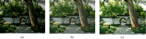
Figure 5. Image enhancement results at different scales
Finally, the image enhancement effects were discussed at different scales. Without changing the other network structural parameters, multiple scales of Gaussian pyramid were adopted to train and test the network. Figure 5 shows the test results. With the growing scale, the image enhancement effect continued to improve, and peaked at the scale of 3.
Based on deep learning and illumination compensation, this paper attempts to develop an effective a multi-scale image enhancement algorithm. Firstly, a compensation algorithm was developed for image illumination drift based on the Hodge decomposition model. Then, the lightweight multi-scale Retinex network was selected to enhance low-illumination multi-scale images, and the network architecture was presented clearly. In addition, a new joint network loss function was designed for the input and output forms, corresponding to the proposed deep learning network, and the low-illumination multi-scale image enhancement. Through experiments, the authors summarized the linear regression coefficients of low-illumination image database before and after illumination compensation, revealing that our algorithm has the best illuminance compensation effect. The authors also compared the image retrieval correctness of low-illumination image database before and after illumination compensation, and demonstrated that Hodge decomposition-based illumination compensation can effectively enhance the accuracy of image identification and retrieval. Moreover, the change curve of image query correctness with the number of iterations was obtained, and multiple models were quantitatively compared on different low-illumination image datasets. The comparison shows that the combination between lightweight multi-scale Retinex network and Hodge can output images with rich details and bright colors, which are in line with human visual perception and aesthetics. Furthermore, the results of the ablation test shows that the joint use of all seven loss terms led to the optimal effect. Finally, the image enhancement effects were discussed at different scales. The results show that our algorithm has the best image enhancement effect at the scale of 3.
The work is supported by S&T Program of Hebei (Grant No.: 21327212D).
[1] Zhao, L.F., Wang, A.L., Wang, B., Lv, X.M. (2017). Image enhancement algorithm based on sub image fusion. Systems Engineering and Electronics, 39(12): 2840-2848. https://doi.org/10.3969/j.issn.1001-506X.2017.12.30
[2] Al-Betar, M.A., Alyasseri, Z.A.A., Khader, A.T., Bolaji, A.L.A., Awadallah, M.A. (2016). Gray image enhancement using harmony search. International Journal of Computational Intelligence Systems, 9(5): 932-944. https://doi.org/10.1080/18756891.2016.1237191
[3] Hao, S., Pan, D., Guo, Y., Hong, R., Wang, M. (2016). Image detail enhancement with spatially guided filters. Signal Processing, 120: 789-796. https://doi.org/10.1016/j.sigpro.2015.02.017
[4] Righi, M., D’Acunto, M., Salvetti, O. (2016). An image enhancement tool: Pattern recognition image augmented resolution. Pattern Recognition and Image Analysis, 26(3): 518-523. https://doi.org/10.1134/S1054661816030160
[5] Walha, R., Drira, F., Lebourgeois, F., Alimi, A.M., Garcia, C. (2016). Resolution enhancement of textual images: a survey of single image-based methods. IET Image Processing, 10(4): 325-337. https://doi.org/10.1049/iet-ipr.2015.0334
[6] Isa, I., Sulaiman, S.N., Abdullah, M.F., Tahir, N.M., Mustapha, M., Karim, N.K.A. (2016). New image enhancement technique for WMH segmentation of MRI FLAIR image. In 2016 IEEE Symposium on Computer Applications & Industrial Electronics (ISCAIE), pp. 30-34. https://doi.org/10.1109/ISCAIE.2016.7575032
[7] Deng, H., Sun, X., Liu, M., Ye, C., Zhou, X. (2016). Image enhancement based on intuitionistic fuzzy sets theory. IET Image Processing, 10(10): 701-709. https://doi.org/10.1049/iet-ipr.2016.0035
[8] Park, S., Kim, K., Yu, S., Paik, J. (2018). Contrast enhancement for low-light image enhancement: A survey. IEIE Transactions on Smart Processing & Computing, 7(1): 36-48. https://doi.org/10.5573/IEIESPC.2018.7.1.036
[9] Feng, Y.Y., Wang, J.P., Ma, S.L., Li, C., Wu, Y. (2018). New COPLIP model and its image enhancement algorithm. Xi'an Dianzi Keji Daxue Xuebao/Journal of Xidian University, 45(1): 66-71.
[10] Wang, Z., Wang, K., Yang, F., Pan, S., Han, Y., Zhao, X. (2018). Image enhancement for crop trait information acquisition system. Information Processing in Agriculture, 5(4): 433-442. https://doi.org/10.1016/j.inpa.2018.07.002
[11] Hu, D., Wu, Z. (2015). Enhancement of degraded image based on neural network. Metallurgical and Mining Industry, (4): 281-287.
[12] Hsieh, P.W., Shao, P.C. (2022). Hue-preserving image enhancement via complementary enhancing terms. Signal Processing, 195: 108491. https://doi.org/10.1016/j.sigpro.2022.108491
[13] Ito, R., Fujita, K. (2017). Image enhancement of cloth stain using ICA. Kyokai Joho Imeji Zasshi/Journal of the Institute of Image Information and Television Engineers, 71(11): J287-J294.
[14] Kapil, D. (2015). Face recognition of blurred images using image enhancement and texture features. In 2015 1st International Conference on Next Generation Computing Technologies (NGCT), pp. 894-897. https://doi.org/10.1109/NGCT.2015.7375248
[15] Chang, H., Ng, M.K., Wang, W., Zeng, T. (2015). Retinex image enhancement via a learned dictionary. Optical Engineering, 54(1): 013107. https://doi.org/10.1117/1.OE.54.1.013107
[16] Tseng, C.C., Lee, S.L. (2017). A weak-illumation image enhancement method uisng homomorphic filter and image fusion. In 2017 IEEE 6th Global Conference on Consumer Electronics (GCCE), pp. 1-2. https://doi.org/10.1109/GCCE.2017.8229192
[17] Sang, Y., Li, T., Zhang, S., Yang, Y. (2022). RARNet fusing image enhancement for real-world image rain removal. Applied Intelligence, 52(2): 2037-2050. https://doi.org/10.1007/s10489-021-02485-1
[18] Yamakawa, M., Sugita, Y. (2018). Image enhancement using Retinex and image fusion techniques. Electronics and Communications in Japan, 101(8): 52-63. https://doi.org/10.1002/ecj.12092
[19] Lee, S., Kim, D., Kim, C. (2018). Ramp distribution-based image enhancement techniques for infrared images. IEEE Signal Processing Letters, 25(7): 931-935. https://doi.org/10.1109/LSP.2018.2834429
[20] Shi, Z., Zhu, M., Guo, B., Zhao, M. (2017). A photographic negative imaging inspired method for low illumination night-time image enhancement. Multimedia Tools and Applications, 76(13): 15027-15048. https://doi.org/10.1007/s11042-017-4453-z
[21] Qi, W., Han, J., Zhang, Y., Bai, L.F. (2016). Hierarchical image enhancement. Infrared Physics & Technology, 76: 704-709. https://doi.org/10.1016/j.infrared.2016.04.010
[22] Xiao, J., Peng, H., Zhang, Y., Tu, C., Li, Q. (2016). Fast image enhancement based on color space fusion. Color Research & Application, 41(1): 22-31. https://doi.org/10.1002/col.21931
[23] Kim, S.E., Jeon, J.J., Eom, I.K. (2016). Image contrast enhancement using entropy scaling in wavelet domain. Signal Processing, 127: 1-11. https://doi.org/10.1016/j.sigpro.2016.02.016
[24] Puniani, S., Arora, S. (2015). Performance evaluation of image enhancement techniques. International Journal of Signal Processing, Image Processing and Pattern Recognition, 8(8): 251-262. http://dx.doi.org/10.14257/ijsip.2015.8.8.27
[25] Ganguli, S., Mahapatra, P.K., Kumar, A. (2015). Artificial immune system based image enhancement technique. In Advances in Intelligent Informatics, 1-8. https://doi.org/10.1007/978-3-319-11218-3_1
[26] Huang, Z., Li, X., Wang, L., Fang, H., Ma, L., Shi, Y., Hong, H. (2022). Spatially adaptive multi-scale image enhancement based on nonsubsampled contourlet transform. Infrared Physics & Technology, 104014. https://doi.org/10.1016/j.infrared.2021.104014
[27] Zhou, D., Qian, Y., Ma, Y., Fan, Y., Yang, J., Tan, F. (2022). Low illumination image enhancement based on multi-scale CycleGAN with deep residual shrinkage. Journal of Intelligent & Fuzzy Systems, 42(3): 2383-2395. https://doi.org/10.3233/JIFS-211664
[28] Zhou, J., Yao, J., Zhang, W., Zhang, D. (2022). Multi-scale retinex-based adaptive gray-scale transformation method for underwater image enhancement. Multimedia Tools and Applications, 81(2): 1811-1831. https://doi.org/10.1007/s11042-021-11327-8
[29] Pan, X.Y., Wei, M., Wang, H., Jia, F.Z. (2022). A multi-scale fusion residual encoder-decoder approach for low illumination image enhancement. Jisuanji Fuzhu Sheji Yu Tuxingxue Xuebao/Journal of Computer-Aided Design and Computer Graphics, 34(1): 104-112. https://doi.org/10.3724/SP.J.1089.2022.18833
[30] Yuan, J., Cai, Z., Cao, W. (2021). TEBCF: Real-world underwater image texture enhancement model based on blurriness and color fusion. IEEE Transactions on Geoscience and Remote Sensing, 60: 1-15. https://doi.org/10.1109/TGRS.2021.3110575