Wei Chen* | Xuan Zheng | Haijun Zhou | Zhe Li
© 2021 IIETA. This article is published by IIETA and is licensed under the CC BY 4.0 license (http://creativecommons.org/licenses/by/4.0/).
OPEN ACCESS
The world is severely impacted by the coronavirus (COVID19). During the epidemic, logistics service, an often-overlooked pillar of the modern society, steps into the spotlight. However, the service capability is inevitably weakened by the epidemic. The fatigued service providers are increasingly unable to meet the high expectations of users, who therefore leave harsh comments on logistics services. It is important for managers to find information that helps to improve management, out of the biased and angry comments. Text sentiment analysis is a fundamental work in natural language processing (NLP). In recent years, graph neural network (GNN) has achieved excellent performance in various NLP tasks. Nevertheless, GNN only considers the adjacent words, as it updates graph nodes. The model thereby emphasizes local features over global features, and misses the intent of the comment text. This paper constructs a triple graph neural network (TGNN) to serve the sentiment analysis of service texts. Firstly, the corresponding node connection windows were applied on different network layers to consider both local and global features. Next, the graph attention network (GAT) was adopted as the message delivery mechanism to fuse the features of all word nodes in the graph. Experimental results show that, the TGNN can evaluate the comment texts on logistics service quality more accurately than the other models.
logistics service quality, text sentiment analysis, attention mechanism, multi-level graph neural network (MLGNN)
As informatization goes deeper, online service provision can slash the cost of logistics management, and provide users a platform to express their personal opinions [1]. These emotional opinions help to identify the problems arising in the service process, and make a reasonable evaluation of the services enjoyed by users. The same service process or outcome is often viewed differently by different users, triggering different personal emotions. Understanding these differences forcefully supports management measures that improve service quality and user experience. To date, sentiment analysis has been widely used in online service evaluation, various recommendation systems, public opinion analysis, and many other fields [2, 3]. For example, it is possible to model user-service relationship through text sentiment analysis on user comments of the logistics service platform, and provides a user-side quantitative model for improving service quality. This is particularly important, because the service-side does not necessarily provide services truly needed by users.
Text sentiment analysis is essentially a text classification task, in which a suitable classification model should be built to classify text contents into predefined emotional polarity, e.g., satisfied, and dissatisfied. There are roughly three kinds of text sentiment analysis methods: dictionary-based methods, shallow learning methods, and deep learning methods.
Dictionary-based methods summarize common emotional words into an emotional dictionary, and matches the input text with the dictionary contents. Then, the emotional words that match the emotional dictionary are found in the text. Finally, the emotional polarity of the text is determined. Esuli and Sebastiani [4] provided an emotional dictionary called SentiWordNet, which contains a predefined vocabulary. By eliminating the need for training, the dictionary-based methods greatly shorten the time for analysis. However, there are several challenges facing these methods: lots of manual labels are needed to build the emotional dictionary; a single vocabulary cannot support cross-domain research; it is difficult to determine the emotional polarity of a text, which contains two or more emotional words.
Shallow learning methods, a.k.a., traditional machine learning [5], focus on feature engineering. They often express texts with sparse word features, the most popular of which are bag-of-words (BOW) [6] and N-gram [7] Based on word frequency statistics, the BOW algorithm has a high computing efficiency. But the order of words is overlooked by the BOW. N-gram outperforms the BOW by capturing some information of the order of the words. The traditional methods depend on various classifiers. Wang and Lin [8] discussed the relationship between feature selection and classification performance. Nonetheless, shallow learning methods seriously rely on manually selected features. The development of such methods is further constrained by the limited expression ability and poor generalization ability of the classifiers. Consequently, more and more researchers have turned to deep learning methods [9, 10].
Word2Vec [11] provides an effective way to learn distributed vocabulary, and underpins the wide application of deep learning methods in text sentiment analysis [12, 13]. The most representative depth neural network for text sentiment analysis is the convolutional neural network (CNN) and recurrent neural network (RNN). Unlike the convolution in computer vision [14], the CNNs in text sentiment analysis are often one-dimensional (1D) [15], which acquires contextual information by mimicking N-grams. To predict the emotions of comments, Wehrmann et al. [16] proposed a language-independent CNN-based character-level world embedding method. Compared with the recurrent model, CNN speeds up learning through parallel operations. But CNN has a low accuracy, because it emphasizes local features over contextual information. By contrast, RNN and its variant long-short-term memory (LSTM) [17] as well as gated recurrent unit (GRU) [18], fully consider the contextual associations, and store more, longer global information, which greatly facilitate text sentiment analysis. Based on LSTM, Ruan [19] put forward a sequential neural encoder with latent structured description (SNELSD), and verified its good effect on datasets like Stanford Natural Language Inference (SNLI) [20] and Standard Sentiment Treebank (SST) [21]. Huang et al. [12] came up with an attention-based modality-gated network (AMGN) to learn the multimodal features for graph and text sentiment analysis. The AMGN adaptively selects the modals of the relatively fierce emotional information to learn multimodal features. Despite being context-aware, LSTM has a highly complex recurrent structure. The dependence of multiple gates and the storage unit on the previous time step linearizes the LSTM operation, making it difficult for the graphic processing unit (GPU) to speed up the computing through parallel computing. The RNN and its variants mainly target continuous word sequences, but do not clearly use the word co-occurrence information. Their complex model structures function like a black box.
The graph neural network (GNN) [22] attracts much attention in text analysis. In the GNN, a node collects information from other nodes, and updates its representation. The GNN has been applied to various natural language processing (NLP) tasks, including text classification [23, 24], neural machine translation (NMT) and relationship reasoning, etc. [25]. Drawing on graph convolutional network (GCN) [26], Yao et al. [23] presented a text classification method called Text_GCN, which constructs a single text graph for the entire corpus based on word co-occurrence and file-word relationship. The defects of Text-GCN are high memory consumption and incompatibility with online test. In addition, the order between words is ignored during the plotting of the text graph. To solve these problems, Huang et al. [24] developed a text-level GNN for text classification (H-GNN). Instead of plotting the entire corpus, the H-GNN builds a graph for each input text. However, the graph nodes are updated only in the light of the adjacent nodes within a small window, without considering the relationship between nonadjacent nodes. Like the CNN, the H-GNN merely stresses local features, and has difficulty in learning the dependence between faraway nodes.
To solve the defects of the above models and benefit the evaluation of texts on logistics service quality, this paper establishes a triple graph neural network (TGNN) for text sentiment analysis, and this is a multi-level graph neural network [27]. Firstly, a graph was generated for every input text, rather than plot a graph for the entire corpus. Next, the model was divided into three layers, mimicking how humans comprehend different layers of languages. The first layer was connected to the word nodes within the small window, the second layer to the word nodes in the large window, and the third layer to all word nodes. To fuse the features of all word nodes in the graph, the scaled dot product attention mechanism [28] was integrated into the TGNN, and connection windows of different sizes were adopted for the first layer and the second layer, aiming to consider both global and local features. Finally, several experiments were carried out on public datasets and a self-developed dataset of texts on logistics service comments. The experimental results show that the TGNN can handle text sentiment analysis better than similar methods, and achieve the best quality in service evaluation.
This section details the structure of the TGNN. Firstly, the authors explained how to build graphs, and describe the message transfer mechanism of the first layer. Next, the authors introduced how to design graph structure, and update the representation of nodes at the second layer, with the help of graph attention network (GAN) [29]. After that, the authors demonstrated how to update the representation of nodes on the third layer, using the scaled dot product attention mechanism. Finally, the authors introduced the output function and loss function of the MLGNN.
2.1 Background
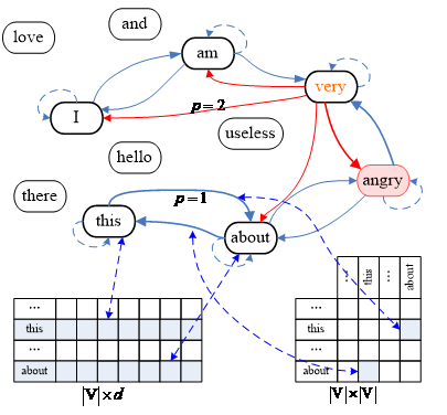
The TGNN is established based on Text-GCN and H-GNN. In the Text-GCN, the nodes starting with file objects and the other nodes are words; connect them with lines if there is a relationship. There are two relationships here: file-word relationships and word-word relationships. This structure maps the entire corpus. In addition to occupying lots of memory, Text-GCN overlooks the order between words, i.e., the context. To a certain degree, the ignorance of the context undermines the final classification accuracy. By contrast, the H-GNN text classification does not establish a single corpus-level graph, but a text-level graph. As shown in Figure 1, H-GNN connects word nodes within a small window of the text, and reflects the word order in a sentence with edge connections. However, when the node representation of the graph is updated, H-GNN only considers the adjacent nodes in the small window, failing to take account of the relationship between non-adjacent nodes. Only focusing local features, the model can hardly learn the dependence between far away nodes.
To solve the above problems, the TGNN generates a text graph containing different connection windows. Three layers of node connections were proposed: the first layer, the second layer, and the third layer. The first layer has a small connection window, focusing on local features; the second layer has a large connection window, focusing on far away features; the third layer connects all word nodes with straight lines, focusing on global features.
2.2 First layer
A graph similar to H-GNN [24] is constructed on the first layer. The text containing l words is represented as $T^{(0)}=\left\{r_{1}^{(0)}, \cdots, r_{i}^{(0)}, \cdots, r_{l}^{(0)}\right\}$, where $r_{i}^{(0)}$ is the representation of the i-th word.$r_{i}^{(0)}$ is initialized by a $d_{0}$-dimensional word embedding, and updated through the training process. For a given text, each word is treated as a graph node. Every edge starts from a word, and ends at the adjacent word. Let p1 be the number of adjacent words of a word. Then, the graph can be defined as:
${{N}^{(0)}}=\{r_{i}^{(0)}|i\in [1,l]\}$ (1)
${{E}^{(0)}}=\{e_{ij}^{(0)}|i\in [1,l];j\in [i-{{p}_{\text{1}}},i+{{p}_{\text{1}}}]\}$ (2)
where, N(0) and E(0) are the node set and edge set of the bottom layer graph.
Figure 1. Structure of H-GNN
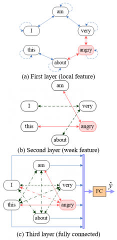
As shown in Figure 2, for the convenience of display, the connection windows of first layer nodes and second layer nodes are denoted as p1=1 and p2=2, respectively.
The message delivery mechanism collects information from adjacent nodes, and update their representation. Since the connection window on the first layer is small, the words in the window are represented similarly. The mean representation of adjacent nodes is solved, and used as the message delivery mechanism on the first layer:
$\hat{r}_{i}^{(1)}=averag{{e}_{a\in N_{i}^{p}}}r_{a}^{(0)}$ (3)
$\tilde{r}_{i}^{(1)}=(1-\beta )\hat{r}_{i}^{(1)}+\beta r_{i}^{(0)}$ (4)
$r_{i}^{(1)}=f({{w}_{bot}}\tilde{r}_{i}^{(1)}+{{b}_{bot}})$ (5)
where, $N_{i}^{p}$ is an adjacent node of the ith node; average is a criterion function that combines the means of all dimensions; $\beta\left(\beta \in R^{1}\right)$ is a configurable parameter indicating how much information should be retained by $R_{i}^{(0)}$. Formula (5) converts node features to a new dimension, where $w_{b o t} \in R^{d_{0} \times d_{1}}$ and $b_{b o t} \in R^{d_{1}}$ are trainable matrices, and f is a nonlinear activation function.
Figure 2. Architecture of the MLGNN
On the bottom layer, the features are firstly collected from adjacent nodes. Then, the node features are updated. Finally, the node representation is converted into a new dimension d1. Since the connection window p is generally a very small value, the bottom layer mainly focuses on the local features of the text.
2.3 Middle layer
In the middle layer, the graph containing l nodes is represented as $T^{(1)}=\left\{r_{1}^{(1)}, \cdots, r_{i}^{(1)}, \cdots, r_{l}^{(1)}\right\}$, where $r_{i}^{(1)}$ is the i-th node. In the middle layer, a large connection window is adopted for the nodes. Let q be the number of adjacent nodes of each node. Then, the graph can be defined as:
${{N}^{(1)}}=\{r_{i}^{(1)}|i\in [1,l]\}$ (6)
${{E}^{(1)}}=\{e_{ij}^{(1)}|i\in [1,l];j\in [i-{{p}_{\text{2}}},i+{{p}_{\text{2}}}]\}$ (7)
where, $N^{(1)}$ is the node set; $E^{(1)}$ is the edge set; p1≤p2.
A large connection window is adopted on the second layer, for the correlations of far away nodes with the current node may vary. Hence, the representations of adjacent nodes cannot be directly averaged, as what is done on the first layer. Here, GAN [29] is employed as the message delivery mechanism of the intermediate layer:
${{c}_{ij}}=\operatorname{LeakyReLU}\left( {{w}_{a}}\left( {{w}_{w}}r_{i}^{\left( 1 \right)}||{{w}_{w}}r_{i}^{\left( 1 \right)} \right) \right)$ (8)
${{a}_{ij}}={\exp \left( {{c}_{ij}} \right)}/{\sum{_{k\in N_{i}^{q}}\exp \left( {{c}_{ik}} \right)}}\;$ (9)
where, || is a series operation; $w_{a} \in \boldsymbol{R}^{2 d_{1}}$ and $w_{w} \in \boldsymbol{R}^{d_{1} \times d_{1}}$ are trainable parameters. Formula (8), a leaky rectified linear unit (LeakyReLU) [30], is a nonlinear function, by which it is possible to compute the correlation coefficient between an adjacent node and the i-th node. Formula (9) is a softmax function. Then, the adjacent node representations are weighed, and converted into new dimensions:
$\hat{r}_{i}^{(2)}=\sum\limits_{j\in N_{i}^{q}}{({{a}_{ij}}{{w}_{w}}r_{j}^{(1)})}$ (10)
$\tilde{r}_{i}^{(2)}=(1-r)\hat{r}_{i}^{(2)}+\gamma r_{i}^{(1)}$ (11)
$r_{i}^{(2)}=f({{w}_{mid}}\tilde{r}_{i}^{(2)}+{{b}_{mid}})$ (12)
where,$\gamma\left(\gamma \in \boldsymbol{R}^{1}\right)$ is a configuration parameter indicating how much information should be retained by $r_{i}^{(1)}$. Next, node features are converted by formula (12) into a new dimension, where $w_{\text {mid }} \in \boldsymbol{R}^{d_{1} \times d_{2}}$ and $b_{\text {mid }} \in \boldsymbol{R}^{d_{2}}$ are trainable matrices, and f is a nonlinear activation function.
2.4 Top layer
On the top layer, the graph containing l nodes can be represented as $T^{(2)}=\left\{r_{1}^{(2)}, \cdots, r_{i}^{(2)}, \cdots, r_{l}^{(2)}\right\}$. To grasp the features of the whole text, all the nodes are interconnected on the top layer. The graph can be defined as:
${{N}^{(2)}}=\{r_{i}^{(2)}|i\in [1,l]\}$ (13)
${{E}^{(2)}}=\{e_{ij}^{(2)}|i\in [1,l];j\in [1,l]\}$ (14)
where, $N^{(2)}$ and $E^{(2)}$ are the node set and edge set of the top layer, respectively.
The multi-head attention mechanism is selected to transfer messages on the top layer. This mechanism is composed of multiple scaled dot-product attention mechanisms. The scaled dot-product attention mechanism can be defined as:
${{c}_{ij}}=\frac{({{w}_{Q}}r_{i}^{(2)}){{({{w}_{k}}r_{j}^{(2)})}^{T}}}{\sqrt{d3}}$ (15)
${{a}_{ij}}=\frac{\exp ({{c}_{ij}})}{\sum{_{k=1}^{l}\exp ({{c}_{ik}})}}$ (16)
$\hat{r}_{i}^{(3)}=\sum{_{j=1}^{l}{{a}_{ij}}({{w}_{v}}r_{j}^{(2)})}$ (17)
where, $w_{Q} \in R^{d_{2} \times d_{3}}, w_{K} \in R^{d_{2} \times d_{3}}$, and $w_{v} \in R^{d_{2} \times d_{3}}$ are trainable parameters. Formula (15) computes the correlation coefficient between any other node and the i-th node.
Suppose there are H scaled dot-product attention mechanisms in the multi-head attention mechanism. Then, we have:
$r_{i}^{(3)}=f({{W}_{0}}(\underset{h=1}{\overset{H}{\mathop{||}}}\,\hat{r}_{ih}^{(3)}))$(18)
where, $w_o \in R^{hd_3×d_3}$ is a trainable matrix; $\hat{r}_{i h}^{(3)}$ is the outcome of the h-th scaled dot-product attention mechanism of the i-thndoe.
2.5 Output
By connecting the node representations outputted by the top layer, we have:
$r=r_{1}^{(3)}||\cdot \cdot \cdot ||r_{i}^{(3)}||\cdot \cdot \cdot ||r_{l}^{(3)}$ (19)
The emotional trend can be obtained through the fully connected layer of softmax:
$\hat{y}=SoftMax({{w}_{pred}}r+{{b}_{pred}})$ (20)
where, $w_{\text {pred }} \in R^{l d_{3} \times c}$ is the trainable matrix mapping vectors to the output space; $b_{\text {pred }} \in R^{c}$ is a trainable bias; c is the number of predefined classes of emotional polarities.
2.6 Loss function
The training goal is to minimize the cross-entropy loss between ground-truth label and predicted label:
$loss=-\sum\limits_{i}^{N}{{{y}_{i}}\log {{{\hat{y}}}_{i}}}$ (21)
where, $y_{i}$ is the i-th ground-truth label; N is the number of samples.
This section describes the experimental setting, and reports the experimental results.
3.1 Datasets
Four datasets were selected to verify the effectiveness of the TGNN. Table 1 shows the statistics on these datasets.
(1) The SST-binary dataset comes from Stanford Sentiment Treebank (SST-fine) [31], a database of movie reviews. The database contains five classes of emotions: strongly positive, positive, neutral, negative, and strongly negative. The SST-binary dataset was constructed entirely based on the same database.
(2) The Sentube-A [32] dataset contains car reviews on YouTube, which are based on videos and ads containing production information. The emotions in the dataset fall into positive and negative classes.
(3) The Sentube-T [33] dataset contains lapthird reviews on YouTube. Similar to Sentube-A, the emotions in Sentube-T fall into positive and negative classes.
(4) Commentary Text on Logistics Service Quality (CTLSQ) is a self-designed dataset of comment texts on college service quality. In total, there are 17,320 samples in all these datasets. Similar to the SST-binary, the CTLSQ contains five classes of emotions: strongly satisfactory, satisfactory, general, dissatisfactory, and strongly dissatisfactory.
Both CTLSQ and SST-binary contain five categories of emotion intensities, so they need to be mapped to binary emotions. The mapping rules are: strongly positive and positive are mapped to positive, strongly negative and negative are mapped to negative, and neutral sentences are deleted.
We divide all datasets into training, validation, and test sets with ratios of 75%, 20%, and 5%.
3.2 Comparative methods
To objectively evaluate the performance of our method in emotional analysis, five models were selected for comparative experiments: Average Variance Extracted (AVE), LSTM, bidirectional LSTM (BiLSTM), CNN, and H-GNN. Among them, AVE is a logistic regression approach, and the other three models are based on neural networks. On the setting of model parameters: (1) AVE is a logistic regression classifier trained by the mean of word embedding of the training samples; (2) LSTM has an embedding layer of different dimensions, which passes the vectors to the LSTM layer. The final hidden state is connected by a 50-dimensional fully connected layer, and then to the softmax layer. The last layer provides the probability distribution of predefined classes. The dropout is set to 0.5. (3) The parameters of BiLSTM are configured similarly as those of LSTM. (4) In CNN, a convolutional layer is connected to the pretrained word embedding. The size of convolutional filters is set to 2, 3, and 4, respectively. Each convolutional layer is followed by a pooling layer. After that, ReLU activation is carried out, and the result is sent to the fully connected layer, which is connected to the final softmax layer. The dropout is set to 0.5. (5) The H-GNN adjust hyperparameters through grid search. The adjacent nodes are connected by 2 windows. Our experiments show that two windows lead to the best performance. The dropout is set to 0.5. (6) The hyperparameters of the TGNN are given in Table 2, where p is the connection window of the first layer, and q is the connection window of the second layer. The dropout is set to 0.5.
After parameter setting, word2vec was adopted to perform 50-, 100-, and 200-dimensional word embedding trainings. Then, the Adam optimizer with the initial learning rate of 1e-3 was adopted. In all experiments, the model that performs the best on the verification set was adopted. The performance of the model on the test set was evaluated. The mean and standard deviation of the test results were selected for analysis.
3.3 Results
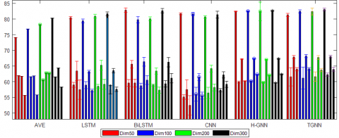
Table 3 reports the experimental results. AVE outperformed LSTM, BiLSTM and CNN on SenTube-A; BiLSTM outperformed LSTM on all datasets; LSTM outperformed BOW and AVE on SST-binary; CNN was outshined by other models on all datasets. Both H-GNN and MLGNN are established on GNN. The results show that GNN-based methods can effectively improve the performance of text sentiment analysis. Specifically, H-GNN outperformed AVE, LSTM, BiLSTM and CNN on H-GNN. Particularly, MLGNN outperformed all the other models on every dataset. MLGNN achieved the highest precision of 300-dimesional word embedding on SST-binary and SenTube-A, and the best accuracy on 100-dimensional word embedding on SenTube-T.
Table 1. Statistics on datasets
|
DataSet |
Training set 75% |
Testing set 20% |
Validation set 5% |
Average sentence length |
Vocabulary |
Labels |
|
CTLSQ |
12990 |
3464 |
866 |
17.30 |
4500 |
2 |
|
SST-binary |
7210 |
1922 |
481 |
19.67 |
17539 |
2 |
|
SenTube-A |
3382 |
900 |
227 |
28.54 |
18569 |
2 |
|
SenTube-T |
4998 |
1333 |
333 |
28.73 |
20276 |
2 |
Table 2. Hyperparameter setting of the TGNN
|
Dataset |
p1 |
p2 |
H |
β |
γ |
d1 |
d2 |
d3 |
|
SST-binary |
1 |
2 |
8 |
0.2 |
0.2 |
200 |
24 |
24 |
|
SenTube-A |
2 |
4 |
8 |
0.2 |
0.2 |
128 |
16 |
16 |
|
SenTube-T |
2 |
3 |
8 |
0.2 |
0.2 |
256 |
40 |
40 |
|
CTLSQ |
2 |
3 |
8 |
0.2 |
0.2 |
256 |
40 |
40 |
Figure 3. Comparison of test results
Table 3. Precisions on different test sets (Dim.300)
|
Method |
SST-binary |
SenTube-A |
SenTube-T |
CTLSQ |
|
AVE |
80.28 |
61.49 |
64.34 |
58.27 |
|
LSTM |
81.67 |
57.41 |
63.51 |
57.58 |
|
BiLSTM |
82.66 |
59.33 |
66.23 |
61.13 |
|
CNN |
81.39 |
57.31 |
62.17 |
59.17 |
|
H-GNN |
82.66 |
59.61 |
67.3 |
62.34 |
|
TGNN |
83.06 |
62.25 |
68.03 |
63.93 |
Table 4. Influence of second and third layers
|
Method |
SST-binary |
SenTube-A |
SenTube-T |
CTLSQ |
|
TGNN/second |
83.0±2.6 |
61.5±1.1 |
66.9±1.2 |
66.9±1.2 |
|
TGNN/ third |
81.9±0.4 |
58.7±0.7 |
67.3±1.1 |
67.3±1.1 |
|
TGNN |
83.1±0.4 |
62.2±0.5 |
68.0±0.4 |
64.0±0.4 |
3.4 Discussion
The influence of high and second layers is reported in Table 4, where MLGNN/second and MLGNN/third refer to MLGNNs without the second layer and the third layer, respectively. MLGNN/second was not as good as TGNN on any dataset, revealing the effectiveness of second- and third-layer text sentiment analyses. MLGNN/third had the worst performance, for failing to extract global features. Considering both local and global features, the TGNN achieved the best performance. In addition, the TGNN explicitly connects adjacent word nodes, and updates node representations by collecting the features of adjacent nodes. This is unachievable by the LSTM.
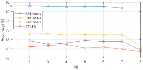
The SST-binary, SenTube-A, SenTube-B, and CTLSQ have 1, 2, 2, and 2 connection windows on the first layer, respectively. Figure 3 shows the influence of q value on model performance.
Figure 4. Influence of q value on model performance
As shown in Figure 4, the model performance degraded when the q value was too large or too small. When $p_{2}=2$, the best performance was observed on SST-binary; when $p_{2}=4$, the best performance was observed on SenTube-A; when $p_{2}=3$, the best performance was observed on SenTube-T; when $p_{2}=5$, the best performance was observed on CTLSQ.The q value stands for the connection window of the second layer. If the p2 value is too small, the second layer will extract the same features as the first layer. If the p value is too large, some features will get lost. Hence, a proper p2 value can improve the performance of TGNN sentiment analysis.
Through accurate text sentiment analysis, it is possible to understand the real emotions of users, and improve the logistic service quality. This paper establishes the MLGNN, a GNN model with connection windows of different sizes. The node representations in the model are updated by different message delivery mechanisms. Specifically, a small connection window is adopted on the bottom layer, and the features of adjacent words are averaged to learn local features; a large connection window is adopted in the middle layer, and the GAN is applied as the message delivery mechanism; all the words in each sentence are connected on the top layer, and the multi-head attention is synthetized to update node features and fuse global features. Experimental results show that MLGNN achieved good precisions on public datasets and a self-designed dataset CTLSQ.
It is worth noting that the MLGNN only represents the order of words in a sentence as edge connections, rather than clarify the sequential relationship. Thus, the model cannot easily handle special sentences like inverted sentences. The future work will consider the positions of encoded nodes in the graph. In addition, the outstanding pretrained language models will be fused with the MLGNN.
This project was funded by the Humanities and Social Science Research Project of Ministry of Education of China (Grant No.: 20YJCZH081), and Scientific Research Project of Education Department of Hubei Province (Grant No.: D20212701, D20202701, B2019389).
[1] Wang, Z., Ho, S.B., Cambria, E. (2020). A review of emotion sensing: categorization models and algorithms. Multimedia Tools and Applications, 79(47): 35553-35582. https://doi.org/10.1007/s11042-019-08328-z
[2] Zhao, S.H., Fu, X.D., Yue, K., Liu, L., Feng, Y., Liu, L.J. (2021). Top-k online service evaluating to maximize satisfaction of user group. Journal of Software, 32(11): 3388-3403. http://dx.doi.org/10.13328/j.cnki.jos.006089
[3] Tan, S., Li, Y., Sun, H., Guan, Z., Yan, X., Bu, J., Chen, C., He, X. (2013). Interpreting the public sentiment variations on twitter. IEEE Transactions on Knowledge and Data Engineering, 26(5): 1158-1170. https://doi.org/10.1109/TKDE.2013.116
[4] Esuli, A., Sebastiani, F. (2006). Sentiwordnet: A publicly available lexical resource for opinion mining. Proceedings of the Fifth International Conference on Language Resources and Evaluation (LREC’06), Genoa, Italy, pp. 417-422.
[5] Haider, S.K., Jiang, A., Jamshed, M.A., Pervaiz, H., Mumtaz, S. (2018). Performance enhancement in P300 ERP single trial by machine learning adaptive denoising mechanism. IEEE Networking Letters, 1(1): 26-29. https://doi.org/10.1109/LNET.2018.2883859
[6] Zhang, Y., Jin, R., Zhou, Z.H. (2010). Understanding bag-of-words model: A statistical framework. International Journal of Machine Learning and Cybernetics, 1(1-4): 43-52. https://doi.org/10.1007/s13042-010-0001-0
[7] Basile, A., Dwyer, G., Medvedeva, M., Rawee, J., Haagsma, H., Nissim, M. (2017). N-gram: New Groningen author-profiling model. arXiv preprint arXiv:1707.03764.
[8] Wang, Z., Lin, Z. (2020). Optimal feature selection for learning-based algorithms for sentiment classification. Cognitive Computation, 12(1): 238-248. https://doi.org/10.1007/s12559-019-09669-5
[9] Zhou, Z., Liao, H., Gu, B., Huq, K.M.S., Mumtaz, S., Rodriguez, J. (2018). Robust mobile crowd sensing: When deep learning meets edge computing. IEEE Network, 32(4): 54-60. https://doi.org/10.1109/MNET.2018.1700442
[10] Aggarwal, A., Rani, A., Sharma, P., Kumar, M., Shankar, A., Alazab, M. (2020). Prediction of landsliding using univariate forecasting models. Internet Technology Letters, e209. https://doi.org/10.1002/itl2.209
[11] Mikolov, T., Sutskever, I., Chen, K., Corrado, G.S., Dean, J. (2013). Distributed representations of words and phrases and their compositionality. Advances in Neural Information Processing Systems, Lake Tahoe Nevada, USA, pp. 3111-3119.
[12] Huang, F., Wei, K., Weng, J., Li, Z. (2020). Attention-based modality-gated networks for image-text sentiment analysis. ACM Transactions on Multimedia Computing, Communications, and Applications (TOMM), 16(3): 1-19. https://doi.org/10.1145/3388861
[13] Xu, J., Li, Z., Huang, F., Li, C., Philip, S.Y. (2020). Social image sentiment analysis by exploiting multimodal content and heterogeneous relations. IEEE Transactions on Industrial Informatics, 17(4): 2974-2982. https://doi.org/10.1109/TII.2020.3005405
[14] Yue, Z., Ding, S., Zhao, L., Zhang, Y., Cao, Z., Tanveer, M., Jolfaei, A., Zheng, X. (2021). Privacy-preserving time-series medical images analysis using a hybrid deep learning framework. ACM Transactions on Internet Technology (TOIT), 21(3): 1-21. https://doi.org/10.1145/3383779
[15] Chen, Y. (2015). Convolutional neural network for sentence classification. Master's thesis, University of Waterloo.
[16] Wehrmann, J., Becker, W., Cagnini, H.E., Barros, R.C. (2017). A character-based convolutional neural network for language-agnostic Twitter sentiment analysis. In 2017 International Joint Conference on Neural Networks (IJCNN), Anchorage, AK, USA, pp. 2384-2391. https://doi.org/10.1109/IJCNN.2017.7966145
[17] Hochreiter, S., Schmidhuber, J. (1997). Long short-term memory. Neural Computation, 9(8): 1735-1780.https://doi.org/10.1162/neco.1997.9.8.1735
[18] Chung, J., Gulcehre, C., Cho, K., Bengio, Y. (2014). Empirical evaluation of gated recurrent neural networks on sequence modeling. arXiv preprint arXiv:1412.3555.
[19] Ruan, Y.P., Chen, Q., Ling, Z.H. (2017). A sequential neural encoder with latent structured description for modeling sentences. IEEE/ACM Transactions on Audio, Speech, and Language Processing, 26(2): 231-242. https://doi.org/10.1109/TASLP.2017.2773198
[20] Bowman, S.R., Angeli, G., Potts, C., Manning, C.D. (2015). A large annotated corpus for learning natural language inference. Proceedings of the 2015 Conference on Empirical Methods in Natural Language Processing, Lisbon, Portugal, pp. 632-642.
[21] Socher, R., Perelygin, A., Wu, J., Chuang, J., Manning, C.D., Ng, A.Y., Potts, C. (2013). Recursive deep models for semantic compositionality over a sentiment treebank. Proceedings of the 2013 Conference on Empirical Methods in Natural Language Processing, Seattle, Washington, USA, pp. 1631-1642.
[22] Scarselli, F., Gori, M., Tsoi, A.C., Hagenbuchner, M., Monfardini, G. (2008). The graph neural network model. IEEE Transactions on Neural Networks, 20(1): 61-80. https://doi.org/10.1109/TNN.2008.2005605
[23] Yao, L., Mao, C., Luo, Y. (2019). Graph convolutional networks for text classification. Proceedings of the AAAI Conference on Artificial Intelligence, 33(1): 7370-7377. https://doi.org/10.1609/aaai.v33i01.33017370
[24] Huang, L., Ma, D., Li, S., Zhang, X., Wang, H. (2019). Text level graph neural network for text classification. Proceedings of the 2019 Conference on Empirical Methods in Natural Language Processing and the 9th International Joint Conference on Natural Language Processing (EMNLP-IJCNLP), Hong Kong, China, pp. 3444-3450. http://dx.doi.org/10.18653/v1/D19-1345
[25] Battaglia, P.W., Pascanu, R., Lai, M., Rezende, D., Kavukcuoglu, K. (2016). Interaction networks for learning about objects, relations and physics. Proceedings of the 30th International Conference on Neural Information Processing Systems, Barcelona Spain, pp. 4509-4517.
[26] Kipf, T.N., Welling, M. (2016). Semi-supervised classification with graph convolutional networks. arXiv preprint arXiv:1609.02907.
[27] Liao, W., Zeng, B., Liu, J., Wei, P., Cheng, X., Zhang, W. (2021). Multi-level graph neural network for text sentiment analysis. Computers & Electrical Engineering, 92: 107096. https://doi.org/10.1016/j.compeleceng.2021.107096
[28] Vaswani, A., Shazeer, N., Parmar, N., Uszkoreit, J., Jones, L., Gomez, A.N., Kaiser, Ł., Polosukhin, I. (2017). Attention is all you need. Advances in Neural Information Processing Systems, Long Beach, CA, USA pp. 5998-6008.
[29] Veličković, P., Cucurull, G., Casanova, A., Romero, A., Lio, P., Bengio, Y. (2017). Graph attention networks. arXiv preprint arXiv:1710.10903.
[30] Clevert, D.A., Unterthiner, T., Hochreiter, S. (2015). Fast and accurate deep network learning by exponential linear units (elus). arXiv preprint arXiv:1511.07289.
[31] Socher, R., Perelygin, A., Wu, J., Chuang, J., Manning, C.D., Ng, A.Y., Potts, C. (2013). Recursive deep models for semantic compositionality over a sentiment treebank. Proceedings of the 2013 Conference on Empirical Methods in Natural Language Processing, Seattle, Washington, USA, pp. 1631-1642.
[32] Uryupina, O., Plank, B., Severyn, A., Rotondi, A., Moschitti, A. (2014). SenTube: A corpus for sentiment analysis on YouTube social media. Proceedings of the Ninth International Conference on Language Resources and Evaluation (LREC'14), Reykjavik, Iceland, pp. 4244-4249.
[33] Barnes, J., Klinger, R., Walde, S.S.I. (2017). Assessing state-of-the-art sentiment models on state-of-the-art sentiment datasets. arXiv preprint arXiv:1709.04219.