Mourad Moussa* | Ali Douik
© 2021 IIETA. This article is published by IIETA and is licensed under the CC BY 4.0 license (http://creativecommons.org/licenses/by/4.0/).
OPEN ACCESS
The edge is the most significant information in image processing applications. Moreover, and the accurate and continue edge commonly leads to accurate related steps like object tracking and region clustering. In fact, it is the first step of image analysis and understanding. The accuracy edge detection results have an impact on the comprehension machine system. In this paper we present various improved edge detection techniques by our research team, of similar color and grey level images, using the information theory approach based on other energy information inspired from Shannon entropy and utilizing as well the metaheuristic and intelligent method combined with multilevel thresholding approach in various color spaces, and like the ant colony optimization with the graph cut approach for indexing images before the segmentation step. In addition, particular swarm optimization is done, and finally the fuzzy technique is used. The effectiveness and accuracy of these approaches are evaluated by many metric measurements and compared with the common operators. The PR metric, has a significant mean value (about 20) than PR of Canny operator (about 9). And also, we can denote that all improved techniques achieve significant results with ameliorated running time.
edge detection, neural network, fuzzy logic, Shannon entropy, conditional entropy, joint entropy, metaheuristic algorithm
In the recent years, edge detection and the ant colony algorithm are the methods used in many computer vision applications such as segmentation [1], binarization [2], feature extraction [3], face recognition [4] and edge detection [5]. Intelligent approaches, based on the swarming behavior of animal colonies in nature, has been used widely and successfully in image processing tools, especially when it comes to edge detection, which is the most difficult task because of the complexity of images. Traditional methods were used for detecting cracks brightened up in bridges by Abdel-Qader et al. [6]. Other studies of edge detection presented for measuring the crack width and detecting cracks on surfaces respectively by Adhikari et al. [7] and Dorafshan et al. [8] and Dorafshan et al. [9]. These studies proved that the common edge detector operator achieved the most accurate crack detection.
Thresholding is one of the most used methods in computer vision applications, but a weak compactness of various distribution representing clusters leads to false detection of edge pixels. This approach suffers from the spatial correlation of images and there are different images having the same histograms that give the same threshold value. however, the running time and the location of the various clusters which delimit the full and continuous edge, present the common and crucial problems in this topic. A lot of studies have been done that remedy to these gaps, Otsu [10], Kittler and Illingworth [11], potential difference [12], max entropy [13, 14], and multilevel threshold [15]. Two ways separate the foreground from the background. The first one is bi-level thresholds in Grayscale Images (GIs) and medical images. The second is based on thresholding and clustering an image into various classes. There are two categories of thresholding technique: parametric and non-parametric [16], (1) determines the optimal thresholds by optimizing inter-class and intra-class variances [17] and (2) requires assuming, for each segmented area, the probability density model and estimating the relevant parameters. Recent studies [18] have proved that the Artificial Bee colony (ABC) can be a suitable tool to find optimum thresholds and edge detection, it's an easy algorithm and has a limited parameters and offering very high robustness [19]. Moreover, metaheuristic algorithms can be the best choice of problem optimization to improve edge detectors. The automatic threshold selection was evaluated by Ye et al. [20] based on the ABC algorithm. Zhang et al. optimize running time using global thresholding based on ABC algorithm [21], in addition Ma et al. operate with the GI to select threshold for image segmentation [22].
In this paper we have proposed many edge detection techniques based on intelligent, statistique, and metaheuristic tools. Therefore, color is the more significant information that ameliorate the compactness of various distribution allowing a high quality thresholding. The metaheuristic algorithms are used on clusters center optimization to obtain more significant color image segmentation. The ABC algorithm is incorporated with the Otsu multi-level thresholding approach which operates with color image converted in Lab, YCbCr, HSL color space. Also ACO algorithm was used with the Graph Cut approach that consists of dividing the image into many regions and minimizing an energy function F(λ) which leads to assign an index to each optimal region. As for the PSO algorithm optimizes the clusters center and provides segmented image in the output. And also we have introduced different type of signal energy like joint and conditional entropy for edge detection. Finally, Fuzzy logic technique have done for the same raison and the robustness was tested by salt & pepper noise. This paper is organized as follows. Section 2 describes edge detection based on the metaheuristic optimization algorithm. Section 3 describes edge detection based on the fuzzy logic and various Shannon entropies. Section 4 discusses the experimental results and shows the robustness of our suggested techniques.
2.1 ABC
In nature, several species are characterized by social behavior. Schools of fish, flocks of birds and flocks of land animals are the result of the biological need that drives them to live in groups. This behavior is also one of the main characteristics of social insects (bees, termites, ants, etc.). From these principles, the researchers have been inspired to develop methods based on the behavior of these animals, which has given birth to metaheuristic methods. This word relates to all methods that model the interaction of agents (animals) that are able to self-organize. They represent combinatorial problem-solving methods that consist in repeating certain processes until the optimal solution is obtained.
One of the most organized and rigorous insects in their work are the bees. They have a very high capacity to communicate. Thanks to their intelligence, a method called the bee method has been developed. In this method, artificial bees represent agents which, by collaborating with each other, solve complex problems of combinatorial optimization. From this information we derive the basic idea of this method: to create a multi-agent system capable of successfully solving complex problems. Our algorithm contains three types of bees: scout bees, employed bees, and onlooker bees.
2.2 Threshold selection and image segmentation
Several studies have been done [23-25] and focused on the color space [26], where authors proposed methods to convert it to numerical values and represented it on a 3D graph, according to Bora and Gupta [27]. The ABC algorithm is applied our work to segment an image into k regions based on Otsu’s technique. Image segmentation consists on: color space conversation, generation of artificial agents in the image, optimum threshold evaluation, image segmentation, and edge detection. The classes designation is focused on Color-histogram-analysis, classes are constructed by analyzing the color histogram H[I] of the image I [28]. To do this, the histograms of each color space components are created, which evaluates the distribution of color intensities of each pixel H[I](p) in the image.
We attribute for each artificial ant one code (three integers from 0 to 255). Hence, the number of optimal thresholds is equal to bee’s number. In order to divide the color sets into k homogeneous color clusters, we will take advantages of the two algorithms ABC and multi-level Otsu to propose a hybrid variant for color clustering. As it’s shown in Figure 1, and also the selection of the optimal thresholds values for each component color space. Finally, the three obtained levels are superimposed to have resulting image.
Figure 1. Segmentation process by optimum thresholding for color image
3.1 ACO
According to Dorigo’s ACO website, "Ant colony optimization studies artificial systems that take inspiration from the behavior of the real ant colonies and which are used to solve discrete optimization problems [29]". Thus, by observing ants during the foraging activity, and then discovering the strategy of these ants to find the shortest track to reach food sources. Then, he imitated and modeled its behavior in searching of the best path in a graph.
The strategy goes like this [30]: When ants are looking for food, going from their nest to food sources, they have decided where to go and which path to take. At first, they find themselves in front of several paths lead to the food source, so they explore it all randomly. During their movements, ants are capable of producing chemicals, known as pheromones, deposited to mark the path on the ground that others can follow. The more they use the shorter selected trail, the most optimal line will become increasingly attractive and the pheromone trail concentration will grow stronger, while decreased by the evaporation phenomenon on the other paths. This is because of some natural factors (temperature and wind). Accordingly, the ants will more likely choose to follow the path with higher pheromone levels.
3.2 ACO Algorithm for optimum clusters selection
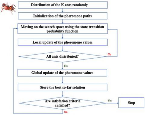
First of all, we have to say that the ant system algorithm is improved to solve the Traveling Salesmen Problem (TSP) [31], which is all about finding the least costing path verifying two conditions: Starting from one point, the salesmen have to go to all other cities just once and come back to the original. Each artificial ant has to find the best solution by moving step by step on the search space states. Figure 2 describes ACO algorithm and summarize the different steps [32]:
$P_{i j}^{k}(t)= \begin{cases}\frac{{\tau_{i j(t)^{\alpha}} \quad \times \eta_{i j}(t)^{\beta}}}{\sum l \in J_{i}^{k} \times {\tau_{i j(t)^{\alpha}} \quad \times \eta_{i j}(t)^{\beta}}} & \text { if } j \in J_{i}^{k} \\ 0 & \text { Otherwise }\end{cases}$ (1)
where, τij(t) is the pheromone trail intensity between the two states i and j, ηil(t) is the heuristic function (visibility), and α and β are two adjustable parameters used to regulate the influence of the pheromone and the visibility. For the TSP, the visibility is inversely proportional to the Euclidean distance between two nodes $\frac{1}{d(i, j)}$.
$\Delta \tau_{i j}^{k}(t)=\left\{\begin{array}{cl}\frac{\mathrm{Q}}{L_{k}(t)} & \text { if }(i, j) \in L_{k}(t) \\ 0 & \text { otherwise }\end{array}\right.$ (2)
$\tau_{i j}(t+n)=(1-\rho) \times \tau_{i j}(t)+\rho \times \Delta \tau_{i j}(t)$ (3)
where, $\rho \in[0,1]$ is the evaporation factor, and it regulates the pheromone reduction.
Figure 2. Flowchart of ACO algorithm organization
$\tau_{i j}(t+n)=(1-\rho) \times \tau_{i j}(t)+\rho \times \tau_{0}$ (4)
Exit: The solution of the algorithm: The best path that it has been found.
3.3 Image segmentation by graph cut
Graph cut methods treat the image segmentation as a label assignment problem. Image I will be divided into homogeneous Nreg regions [34, 35] that respect some of the image characteristics (intensity, color…). Each region Rl is represented by a group of pixels, whose have a similar border and one label l. In this case, the segmentation is performed via minimizing an energy function [36] expressed by Eq. (5):
$F(\lambda)=D(\lambda)+\gamma R(\lambda)$ (5)
where, λ is an indexing function that assigns each pixel of image I to a region. Eq. (6) and (7) respectively represent the D measure that calculates the disagreement between the intensity of pixels in each segment and the segment representative intensity, and R measures the difference between the intensity of pixels from each other in each segment, and γ is a positive constant regularizing coefficient that controls the relative importance of first and second terms.
$D(\lambda)=\sum_{l \in L} \sum_{p \in R_{l}}\left(\mu_{l}-I_{p}\right)^{2}$ (6)
where, Rl [37] is the average of intensity values of the pixels in segment l, and μl is the intensity representative of Rl.
$R(\lambda)=\sum_{p, q \in N} r(\lambda(p), \lambda(q))$ (7)
where, N a neighborhood group that contains all pairs of neighboring pixels, and $r(\lambda(p), \lambda(q))$ is a smoothness regularization function given by the truncated squared absolute difference. Let $G=\{V, E\}$ be a weighted graph, where V is a group of vertices and edges link between them, and $G^{\prime}=\left\{V^{\prime}, E^{\prime}\right\}$ be a cut, where $E^{\prime} \subset E$ is a partition of vertices into two subsets (source and the sink) in the induced graph with separate terminals [38].
3.4 Determination of optimum cluster centers using ACO
Now let us incorporate the ACO algorithm with the graph cut approach for image segmentation. Firstly, we have to define the states of the environment in which the ant colony lives. Hence, the discrete space, where the artificial ants move and try to find a solution, is defined by the pixels of the image with a size of M×N, and the food is the edge pixels.
3.4.1 Initialization process
Aydin and Uğur [39] created the three histograms of the three-dimensional color spaces, and then they gathered the center points of bins. x, y and z are the bin center sets:
$x=\left\{x_{1}, x_{2}, \ldots, x_{n}\right\} \quad y=\{y 1, y 2, \ldots, y n\} \quad z=\{z 1, z 2, \ldots, z n\}$
where, n is the number of bins in histograms xi, and yi and zi are the centers of each bin. The combination of these three bin center sets defines the candidate cluster center point set. Moreover, the search space is defined by the following expression: $S=\{(x 1, y 1, z 1),(x 1, y 1, z 2), \ldots,(x n, y n, z n)\}$.
3.4.2 Heuristic function
The visibility of pixels at position (i, j) is defined by Eq. (8):
$\mu_{i j}=V_{c}\left(I_{i, j}\right) / Z$ (8)
where, $Z=\sum_{i=1}^{m} \sum_{j=1}^{n} \operatorname{Vc}(I i, j)$ is a normalization factor and I(i, j) is the pixel value at position (i, j), and Vc(Ii, j) (Figure 3) is the function of a window of pixels with a size of 3×3 which can be measured with Eq. (9):
Figure 3. Computation of variation Vc(Ii, j) at I(i, j) pixel position defined in Eq. (9)
$V_{c}\left(I_{i, j}\right)=f\left(\left|\mathrm{I}_{-1}-1, \mathrm{j}-1-\mathrm{I}_{\mathrm{i}}+1, \mathrm{j}+1\right|\right.$
$\left.+\left|\mathrm{I}_{\mathrm{i}-1, \mathrm{j}+1}-\mathrm{I}_{\mathrm{i}+1, \mathrm{j}-1}\right|+\ldots+\left|\mathrm{I}_{\mathrm{i}-1, \mathrm{j}}-\mathrm{I}_{\mathrm{i}+1, \mathrm{j}}\right|\right)$ (9)
The f() function is determined by Eq. (10):
$f(x)= \begin{cases}\sin \left(\frac{\pi x}{2 \lambda}\right) \lambda x i f j \in J_{i}^{k} \\ 0 & \text { else }\end{cases}$ (10)
where, λ adjusts the function shape, as shown in Figure 3.
3.4.3 Ants’ solution construction process
Unlike the original ACO, this approach has some differences:
$f=\frac{\sum_{i=1}^{m} \sum_{j=1}^{n} \min \left(\operatorname{dist}\left(p_{i}, C_{j}\right)\right)}{N}$
$+\frac{M \times \max (M) \times \ln (M)}{n}$ (11)
where, N represents the number of bins in a histogram, M represents the number of cluster centers in an ant solution, pi is a pixel, Cj is the cluster center in the ant solution, and max(M) is the maximum number of cluster centers that can be in a solution. After determining the cluster centers by the ACO method, the labels are fixed. Then we apply the graph cut method.
3.4.4 Graph cut method and edge detection
Our objective here is to find the cut with the smallest cost. Based on the pixels’ information of the image, we set the weight of the graph. Then we measure the minimum cost cuts which are the minimum of the energy function, i.e. the sum of the image edge weights. This method can simply identify multiple regions simultaneously, unlike other methods where we have to segment the image into a foreground and a background, repeatable until reaching a stop criterion (no further segment). Finally, in each iteration, the graph cut method directly improves the boundary of identified segments.
4.1 PSO algorithm description
Since the introduction of (PSO) [40], many modifications to the original algorithm have been proposed (Algorithm 1). In many cases, the modifications can be seen as a contribution that provides an improved performance. Indeed, in the ACO algorithm, the n particles constituent the swarm change their states according three conditions: (1) keeping its inertia, (2) changing the condition according to its best position, and (3) changing the condition according to the swarm’s most optimist position. In fact, each particle has its current speed and position evaluated by Eq. (12) and Eq. (13), the most optimized position of each individual and the most optimized position in its neighbourship.
$Vt+1=C1t+C2(Pbest-Pcurrent)+C3(Vbest-Vcurrent)$ (12)
$X_{t+1}=X_{t}+V_{t+1}$ (13)
Algorithm 1:
|
Algorithm of PSO |
|
Input: Swarm size. For each particle - Initialize particle position. - Calculate its fitness. - Take its best position Pcurrent like an initial position. - If f (Pcurrent) < f (Pglobal) -Update the best position of the swarm - Initialize the particle velocities. - Update the global best position Vbest. While Itermaxnot reached do For each particule - Take randomly C2 and C3 values according to the normal distribution in [0, 1]. - Update particule velocities according to Eq. 12. - Update X (t) position according equation 13. - If $f($ Pbest $)<f($ Pcurrent $)$ - Update the best particle position. - If $f($ Pbest $)<f($ Vbest $)$ - Update the best position of the swarm. Output: Vbest: the best position evaluated by the swarm. |
4.2 PSO algorithm for selection of optimum clusters
Initially, each particle represents a probabilistic center of all classes. Therefore, we have total n classes which are the number of agents. We centralize a window around pixels pi and we calculate their membership degrees to classes.
$u_{c i}=\frac{1}{\sum_{l=1}^{k}\left(\frac{\left\|\vec{X}_{i}-\vec{C}_{c}\right\|}{\left\|\vec{X}_{i}-\vec{C}_{l}\right\|}\right)^{\frac{2}{m-1}}}$
$D_{c i}=U_{c i \times} \left\|\vec{X}_{i}-\vec{C}_{c}\right\|$
Then, we evaluate the best local position of particle Plp by the Xie Beni technique: We calculate the pixel deviation value pi related to center C where the particles converge towards a local minimum. As for the best overall position, we don’t take the position of swarm particle with the highest fitness value. However, we apply a new method which selects all particles positions having a value greater than previous global position, or they are called candidates. Each of them has a value called "beta". This parameter is incremented if the current fitness value is higher than its previous one. Finally, the candidate with the highest beta value will be the new best overall position.
Our technique is built on these steps: A 3×3 mask is designed to extract the values of neighbor pixels in each treated image. The inputs of our fuzzy system are based on pixel values and the variation between all pixel against the center pixel. These values are divided under fuzzy subsets. Fuzzy inference rules are defined to decide the partnership of this pixel if it is a boundary or not. The defuzzification step is made by Mamdani’s system, when the resulting output of the fuzzy system is calculated by the centroid method.
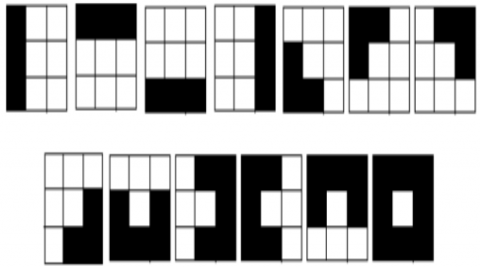
We have used trapezoidal and triangular membership function respectively for fuzzy inputs and outputs. Two fuzzy linguistic variables for inputs (black and white), as well as two fuzzy linguistic variables for outputs (black and edge), are utilized. In our edge detection technique, the inference rules are used to calculate the value of the center pixel based on neighboring pixels. We have used Mamdani fuzzy system which contains 13 rules defining S as an edge pixel, like depicted in Figure 4; i.e., all represented cases confirm the partnership of S to the edge pixels.
Figure 4. Graphical evaluation of rules
Many studies have been based on the mathematical approach for edge detection based on Laplacian and gradient operators. The Shannon entropy is the familiarized approach used by a lot of researchers in several applications like boundary detection [41, 42] image conversion [43] manufacturing industry [44] and information theory [45, 46]. Mohamed El-Sayed et al. [47] proposed an algorithm where two kinds of entropy were incorporated, for edge detection using split and merge techniques.
Besides the analysis of correlation between color levels, the entropy energy metrics have been used as filters of several kernel functions to detect edges in image sequences. The main contribution in this subsection is edge detection in color images checking the robustness of suggested techniques is done by adding noise (salt-and-pepper) with different degrees. In fact, each pixel has three values. For this reason, we operate with the joint entropy and the conditional entropy for two color levels in order to obtain a new entropic matrix of the processed image. The main purpose through this method is to cluster a given image into limited regions. The Shannon entropy metric is given by Eq. (14).
$H=-\sum_{i=0}^{N-1} p_{i} \log _{2} p_{i}$ (14)
The measurements of the joint and conditional entropies are given, respectively, by Eq. (15) and Eq. (16). We evaluate their robustness on boundary detection against noise produced by many issues related to camera displacement and stochastic disturbances.
$H(X, Y)=-\sum_{i=1}^{N} \sum_{j=1}^{M} p\left(X_{i}, Y_{j}\right) \log _{2} p\left(X_{i}, Y_{j}\right)$ (15)
$H(X, Y)=-\sum_{i=1}^{n} \sum_{j=1}^{m} p\left(X_{i}, Y_{j}\right) \log _{2} p\left(X_{i} \mid Y_{j}\right)$ (16)
where, N and M are the size of X, Y, and n, m are the states of these vectors at a given time.
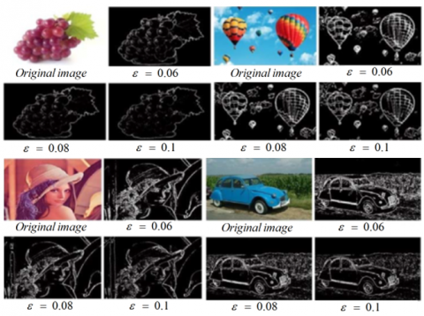
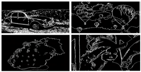
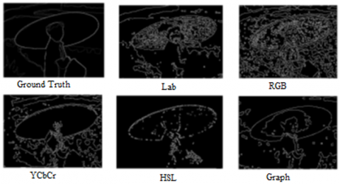
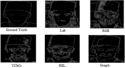
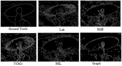
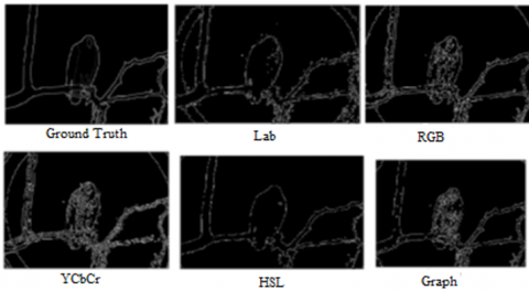
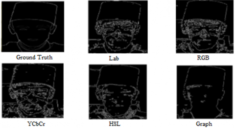
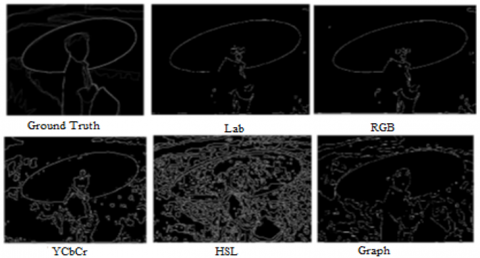
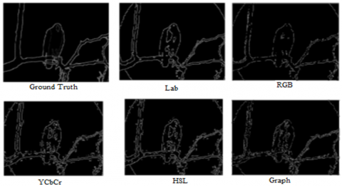
This section describes, presents, evaluates and discusses the results elaborated by the developed technique based on Shannon's entropy information (Figure 5 and Figure 6), metaheuristic approach (Figure 13, Figure 14 and Figure 15) and by the fuzzy logic technique (Figures 10, 11 and 12). Furthermore, we have checked and confirmed the robustness and effectiveness of our approaches by introducing different levels of salt-and pepper noise, as illustrated in Figure 10. Our contributions use various color level. The results of the conditional entropy (Figures 7 and 9) show the impact and the relationship between color levels, and the higher quality results compared to the joint entropy (Figure 8). The RGB color space are excellent: They are accurate to original images and offer a good quality of discrimination. All the image details are also directly identifiable. The edge detection results of these images on the Lab color space are acceptable but not so accuracy.
Figure 5. Results by thresholding method based on Shannon entropy
Figure 6. Edge detection results based on Shannon entropy
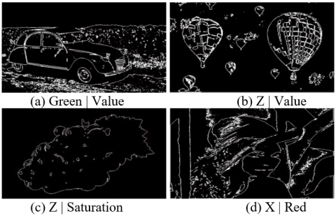
Figure 7. Edge detection results based on conditional entropy
The following parameters are used in all experiments: number of bees = 5, number of iterations =50, limit=100. Figure 13, shows that image represented in YCbCr color space have crucial edge detection than other systems. The edge detection in the HSL color space does not give promising results: many details are missed in treated images or indiscernible, and have a blurred quality. Tables 1, 2 and 3 present the performance metrics of our approach and other algorithms. Our processing method has operated with these parameters: number of ants = 5, number of iterations = 20, α=1, β=0.1, ρ=0.1, number of bins = 15 and max(k)=15. Compared to the Canny method and the ACO technique with gray level, the obtained results are better and have a relevant quality. The PSNR and PR values of our new approach prove this amelioration. After analyzing all the results. we can say that an edge detection image (Figure 10) is improved by our new approach and is better than results using gray-scale images. It gives also good results compared to Canny method, even with various levels of noise and while having reduced running time.
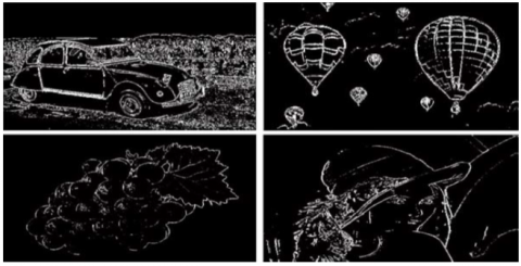
Figure 8. Edge detection results based on joint entropy.
Figure 9. Edge detection results based on conditional entropy
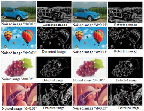
Figure 10. Results of fuzzy method based on pixel value with Salt & pepper noise
Figure 11. Results of fuzzy method based on pixel difference
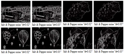
Figure 12. Edge detection based on pixel difference with Salt & pepper noise
(Image 1)
(Image 2)
(Image 3)
Figure 13. Results by ABC algorithm
Figure 14. Results by PSO algorithm
Figure 15. Results by ACO algorithm
Table 1. Segmentation quality evaluation of first image in various color space
|
Image1 |
|
PSNR |
PR |
KI |
|
ACO |
RGB |
20.102 |
14.5226 |
0.031319 |
|
Lab |
20.1194 |
13.9676 |
0.028918 |
|
|
YCbCr |
20.1657 |
18.602 |
0.047572 |
|
|
HSL |
20.2475 |
20.4513 |
0.086828 |
|
|
Graph |
20.2318 |
22.5022 |
0.059706 |
|
|
ABC |
RGB |
19.8441 |
13.0173 |
0.034233 |
|
Lab |
20.0092 |
16.8087 |
0.052068 |
|
|
YCbCr |
19.9892 |
20.906 |
0.057657 |
|
|
HSL |
20.2853 |
17.0431 |
0.044631 |
|
|
Graph |
19.882 |
18.467 |
0.042706 |
|
|
PSO |
RGB |
20.3155 |
23.0107 |
0.078478 |
|
Lab |
20.358 |
18.6794 |
0.079099 |
|
|
YCbCr |
20.3711 |
20.0097 |
0.081023 |
|
|
HSL |
20.2494 |
25.5014 |
0.080005 |
|
|
Graph |
20.1967 |
19.4843 |
0.045541 |
|
|
Canny |
GI |
20.9795 |
8.993 |
0.0240 |
Table 2. Segmentation quality evaluation of second image in various color space
|
Image2 |
|
PSNR |
PR |
KI |
|
ACO |
RGB |
20.1599 |
40.9892 |
0.063578 |
|
Lab |
19.934 |
43.6167 |
0.059654 |
|
|
YCbCr |
19.994 |
42.7968 |
0.065652 |
|
|
HSL |
19.9928 |
43.0419 |
0.065833 |
|
|
Graph |
20.2247 |
48.7938 |
0.076461 |
|
|
ABC |
RGB |
20.2788 |
48.4536 |
0.062765 |
|
Lab |
20.2858 |
47.8476 |
0.071953 |
|
|
YCbCr |
19.867 |
41.0454 |
0.055212 |
|
|
HSL |
20.1391 |
43.8474 |
0.05215 |
|
|
Graph |
19.9497 |
48.1767 |
0.061586 |
|
|
PSO |
RGB |
20.1767 |
52.4819 |
0.085995 |
|
Lab |
20.18 |
45.5655 |
0.08047 |
|
|
YCbCr |
20.2999 |
49.6305 |
0.090228 |
|
|
HSL |
20.0291 |
50.6927 |
0.068234 |
|
|
Graph |
20.1572 |
56.4425 |
0.071322 |
|
|
Canny |
GI |
17.9737 |
14.8333 |
0.0257 |
Table 3. Segmentation quality evaluation of third image in various color space
|
Image3 |
|
PSNR |
PR |
KI |
|
ACO |
RGB |
20.1908 |
31.7029 |
0.062162 |
|
Lab |
20.2435 |
40.2966 |
0.072934 |
|
|
YCbCr |
19.9513 |
27.6958 |
0.048376 |
|
|
HSL |
20.0136 |
20.8201 |
0.041178 |
|
|
Graph |
20.004 |
29.5165 |
0.055206 |
|
|
ABC |
RGB |
20.2727 |
47.6064 |
0.093476 |
|
Lab |
20.2695 |
31.948 |
0.094167 |
|
|
YCbCr |
20.1583 |
35.1403 |
0.086698 |
|
|
HSL |
20.2436 |
25.6176 |
0.056644 |
|
|
Graph |
20.1642 |
13.0635 |
0.032624 |
|
|
PSO |
RGB |
20.4076 |
29.2839 |
0.084146 |
|
Lab |
20.4869 |
30.6345 |
0.079741 |
|
|
YCbCr |
20.2847 |
34.3629 |
0.097192 |
|
|
HSL |
20.0964 |
47.6064 |
0.093476 |
|
|
Graph |
20.2436 |
25.6176 |
0.056644 |
|
|
Canny |
GI |
20.9795 |
8.993 |
0.0203 |
In this paper, we have proposed a very crucial topic of computer vision field, it’s the edge detection application based on several approaches like the Shannon, joint and conditional entropies, on the one hand, and the intelligent and metaheuristic technique and the fuzzy logic method, on the other hand. Our results confirm that the quantity of information energy is an efficient tool for detecting edge. In addition, the highlighting of the various color spaces contributes to maximize the cost function criterion, indeed the most relevant color levels play a crucial role in boundary detection methods especially in the joint and conditional entropies case. Accordingly, our study has investigated the relationship between the different color levels according to the entropy in order to find the best edge detection results. The effectiveness and robustness of our suggested techniques has been confirmed by blurring image by several degree of salt-and-pepper noise. After that, our algorithm has been tested on several images of Berkeley and other databases. In our proposed tools, we have been increasing the segmentation quality of considered image sequences, and also improving the edge detection results as shown in tables above, the PR metric measurements compared with proposed literature algorithms proved that our techniques are very effectiveness and very robustness against the noise than Canny technique. In addition, we have remedied the problems of edge discontinuities, increasing the compactness of various distributions corresponding to the different objects in order to have an optimal thresholding step. The experimental results have shown that our algorithm is highly efficient in terms of running Time and edge detection quality. By using different color spaces in the search area, our algorithm can be successfully applied to multi-level image thresholding rather than boundary detection. In addition, we have proved the impact of incorporating the ACO algorithm and the graph cut approach in the robustness of evaluated results. Many edge detection techniques are conceivable in future research works, like segmentation by classification based on Convolutional Neural Network (CNN), Fuzzy-Neural Network method and also as an extension of proposed metaheuristic techniques, difference evolution can be used.
[1] PirahanSiah, F., Abdullah, S.N.H.S., Sahran, S. (2014). Adaptive image thresholding based on the peak signal-to-noise ratio. Research Journal of Applied Sciences, Engineering and Technology, 8(9): 1104-1116. https://doi.org/10.19026/rjaset.8.1074
[2] Pirahansiah, F., Huda Sheikh Abdullah, S.N., Sahran, S. (2013). Peak signal-to-noise ratio based on threshold method for image segmentation. Journal of Theoretical & Applied Information Technology.
[3] Naeimizaghiani, M., PirahanSiah, F., Abdullah, S.N.H.S., Bataineh, B. (2013). Character and object recognition based on global feature extraction. Journal of Theoretical and Applied Information Technology, 54: 109-120.
[4] Moussa, M., Hmila, M., Douik, A. (2018). A novel face recognition approach based on genetic algorithm optimization. Studies in Informatics and Control, 27(1): 127-134. https://doi.org/10.24846/v27i1y201813
[5] Moussa, M., El Ouni, H., Douik, A. (2020). Edge detection based on fuzzy logic and hybrid types of Shannon entropy. Journal of Circuits, Systems and Computers, 29(14): 2050227. https://doi.org/10.1142/S0218126620502278
[6] Abdel-Qader, I., Abudayyeh, O., Kelly, M.E. (2003). Analysis of edge-detection techniques for crack identification in bridges. Journal of Computing in Civil Engineering, 17(4): 255-263. https://doi10.1061/(ASCE)0887-3801(2003)17:4(255)
[7] Adhikari, R.S., Moselhi, O., Bagchi, A. (2014). Image-based retrieval of concrete crack properties for bridge inspection. Automation in Construction, 39: 180-194. https://doi.org/10.1016/j.autcon.2013.06.011
[8] Dorafshan, S., Maguire, M., Chang, M. (2017). Comparing automated image-based crack detection techniques in the spatial and frequency domains. In 26th ASNT Research Symposium, pp. 34-42.
[9] Dorafshan, S., Thomas, R.J., Maguire, M. (2018). Comparison of deep convolutional neural networks and edge detectors for image-based crack detection in concrete. Construction and Building Materials, 186: 1031-1045. https://doi.org/10.1016/j.conbuildmat.2018.08.011
[10] Otsu, N. (1979). A threshold selection method from gray-level histograms. IEEE Transactions on Systems, Man, and Cybernetics, 9(1): 62-66. https://doi.org/10.1109/TSMC.1979.4310076
[11] Kittler, J., Illingworth, J. (1986). Minimum error thresholding. Pattern Recognition, 19(1): 41-47. https://doi.org/10.1016/0031-3203(86)90030-0
[12] Acharya, J., Sreechakra, G. (1999). Potential Difference Based on Electrostatic Binarization Method.
[13] Pun, T. (1980). A new method for grey-level picture thresholding using the entropy of the histogram. Signal Processing, 2(3): 223-237. https://doi.org/10.1016/0734-189X(85)90125-2
[14] Kaur, A., Verma, K., Bhondekar, A.P., Shashvat, K. (2020). Comparison of classification models using entropy based features from sub-bands of EEG. Traitement du Signal, 37(2): 279-289. https://doi.org/10.18280/ts.370214
[15] Arora, S., Acharya, J., Verma, A., Panigrahi, P.K. (2008). Multilevel thresholding for image segmentation through a fast statistical recursive algorithm. Pattern Recognition Letters, 29(2): 119-125. https://doi.org/10.1016/j.patrec.2007.09.005
[16] Akay, B. (2013). A study on particle swarm optimization and artificial bee colony algorithms for multilevel thresholding. Applied Soft Computing, 13(6): 3066-3091. https://doi.org/10.1016/j.asoc.2012. 03 072
[17] Sarkar, S., Das, S., Chaudhuri, S.S. (2015). A multilevel color image thresholding scheme based on minimum cross entropy and differential evolution. Pattern Recognition Letters, 54: 27-35. https://dx.doi.org/10.1016/j.patrec.2014.11.009
[18] Moussa, M., Guedri, W., Douik, A. (2020). A novel metaheuristic algorithm for edge detection based on artificial bee colony. Traitement du Signal, 37(3): 405-412. https://doi.org/10.18280/ts.370307.
[19] Sharma, T.K., Pant, M. (2017). Shuffled artificial bee colony algorithm. Soft Computing, 21(20): 6085-6104. https://dx.doi.org/10.1007/s00500-016-2166-2
[20] Ye, Z., Hu, Z., Wang, H., Chen, H. (2011). Automatic threshold selection based on artificial bee colony algorithm. 3rd International Workshop on Intelligent Systems and Applications, Wuhan, China, pp. 1-4. http://dx.doi.org/10.1109/ISA.2011.5873357
[21] Zhang, Y., Wu, L. (2011). Optimal multi-level thresholding based on maximum tsallis entropy via an artificial bee colony approach. Entropy, 13: 841-859. http://dx.doi.org/10.3390/e13040841
[22] Ma, M., Liang, J., Guo, M., Fan, Y., Yin, Y. (2011). SAR image segmentation based on artificial bee colony algorithm. Applied Soft Computing, 11(8): 5205-5214. http://dx.doi.org/10.1016/j.asoc.2011.05.039
[23] Zolfaghari, M., Yazdi, M. (2014). A new edge-preserving algorithm based on the CIE-Lu'v'color space for color contrast enhancement. Turkish Journal of Electrical Engineering & Computer Sciences, 22(4): 990-1006. https://doi.org/10.3906/elk-1207-7
[24] Khattab, D., Ebied, H.M., Hussein, A.S., Tolba, M.F. (2014). Color image segmentation based on different color space models using automatic GrabCut. The Scientific World Journal. pp. 1-10. https://doi.org/10.1155/2014/126025
[25] Poynton, C.A. (2012). Digital video and hdtv: Algorithms and interfaces. Morgan Kaufmann. ISBN: 1-55860-792-7
[26] Bora, D.J., Gupta, A.K., Khan, F.A. (2015). Comparing the performance of L* A* B* and HSV color spaces with respect to color image segmentation. arXiv preprint arXiv:1506.01472.
[27] Bora, D.J., Gupta, A.K. (2015). A novel approach towards clustering based image segmentation. arXiv preprint arXiv:1506.01710.
[28] Staal, J., Abràmoff, M.D., Niemeijer, M., Viergever, M. A., Van Ginneken, B. (2004). Ridge-based vessel segmentation in color images of the retina. IEEE Transactions on Medical Imaging, 23(4): 501-509. https://doi.org/10.1109/TMI. 2004.825627
[29] Blum, C. (2005). Ant colony optimization: Introduction and recent trends. Physics of Life Reviews, 2(4): 353-373. https://doi.org/10.1016/j.plrev.2005.10.001
[30] Duan, P., Yong, A.I. (2016). Research on an improved ant colony optimization algorithm and its application. International Journal of Hybrid Information Technology, 9(4): 223-234.
[31] Odili, J.B., Mohmad Kahar, M.N. (2016). Solving the traveling salesman’s problem using the African buffalo optimization. Computational Intelligence and Neuroscience, 37(2016): 1-12. https://doi.org/10.1155/2016/1510256
[32] Khan, S., Bianchi, T. (2018). Ant Colony Optimization (ACO) based data hiding in image complex region. International Journal of Electrical & Computer Engineering, 8(1): 379-389. https://doi.org/10.11591/ijece. v8i1
[33] Brand, M., Masuda, M., Wehner, N., Yu, X.H. (2010). Ant colony optimization algorithm for robot path planning. In 2010 International Conference on Computer Design and Applications, 3: V3-436.
[34] Salah, M.B., Mitiche, A., Ayed, I.B. (2010). Multiregion image segmentation by parametric kernel graph cuts. IEEE Transactions on Image Processing, 20(2): 545-557. https://doi.org/10.1109/TIP.2010.2066982
[35] Wu, H., Sun, X.Y., Liu, Y.N., Wang, D.G., Wei, B. (2020). Fusion between shape prior and graph cut for vehicle image segmentation. Traitement du Signal, 37(2): 255-262. https://doi.org/10.18280/ts.370211
[36] Hofmann, T., Puzicha, J., Buhmann, J.M. (1998). Unsupervised texture segmentation in a deterministic annealing framework. IEEE Transactions on Pattern Analysis and Machine Intelligence, 20(8): 803-818. https://doi.org/10.1109/34.709593
[37] Salah, M.B., Mitiche, A., Ayed, I.B. (2008). A continuous labeling for multiphase graph cut image partitioning. International Symposium on Visual Computing. Springer, pp. 268-277. https://doi.org/10.1007/978-3-540-89639-5_26
[38] Dai, S., Lu, K., Dong, J., Zhang, Y., Chen., Y. (2015). A novel approach of lung segmentation on chest CT images using graph cuts. Neurocomputing, 168(30): 799-807. https://doi.org/10.1016/j.neucom.2015.05.044
[39] Aydın, D., Uğur, A. (2011). Extraction of flower regions in color images using ant colony optimization. Procedia Computer Science, 3: 530-536. https://doi.org/10.1016/j.procs.2010.12.088
[40] Kennedy, J., Eberhart, R. (1995). Particle swarm optimization. In Proceedings of ICNN'95-International Conference on Neural Networks, 4: 1942-1948.
[41] Bukhari, S.U.K., Brad, R., Zamfirescu, C.B. (2014). Fast edge detection algorithm for embedded systems. Stud. Inf. Control, 23: 163-170. http://dx.doi.org/10.24846/v23i2y201404
[42] Fabijańska, A. (2012). A survey of subpixel edge detection methods for images of heat-emitting metal specimens. International Journal of Applied Mathematics and Computer Science, 22: 695-710. http://dx.doi.org/10.2478/v10006-012-0052-3
[43] Hassanien, A.E., Abdelfattah, M., Amin, K.M., Mohamed, S. (2015). A novel hybrid binarization technique for Images of Historical Arabic Manuscripts. Studies in Informatics and Control, 24(3): 271-282. http://dx.doi.org/10. 24846/v24i3y201504
[44] Skubalska-Rafajłowicz, E. (2008). Local correlation and entropy maps as tools for detecting defects in industrial images. International Journal of Applied Mathematics & Computer Science, 18(1): 41-47. http://dx.doi.org/10.2478/v10006-008-0004-0
[45] Andreica, M.E., Dobre, I., Andreica, M.I., Resteanu, C. (2010). A new portfolio selection method based on interval data. Studies in Informatics and Control, 19(3): 253-262. http://dx.doi.org/10.24846/v19i3y201005
[46] Gorecki, H. (2000). Relationship between energy and information. International Journal of Applied Mathematics and Computer Science, 10: 405-411.
[47] El-Sayed, M.A., Bahgat, S.F., Abdel-Khalek, S. (2013). Novel approach of edges detection for digital images based on hybrid types of entropy. Applied Mathematics & Information Sciences, 7(5): 1809. http://dx.doi.org/10.12785/amis/ 070519