Yasasvy Tadepalli | Meenakshi Kollati | Swaraja Kuraparthi* | Padmavathi Kora
© 2021 IIETA. This article is published by IIETA and is licensed under the CC BY 4.0 license (http://creativecommons.org/licenses/by/4.0/).
OPEN ACCESS
Monocular depth estimation is a hot research topic in autonomous car driving. Deep convolution neural networks (DCNN) comprising encoder and decoder with transfer learning are exploited in the proposed work for monocular depth map estimation of two-dimensional images. Extracted CNN features from initial stages are later upsampled using a sequence of Bilinear UpSampling and convolution layers to reconstruct the depth map. The encoder forms the feature extraction part, and the decoder forms the image reconstruction part. EfficientNetB0, a new architecture is used with pretrained weights as encoder. It is a revolutionary architecture with smaller model parameters yet achieving higher efficiencies than the architectures of state-of-the-art, pretrained networks. EfficientNet-B0 is compared with two other pretrained networks, the DenseNet-121 and ResNet50 models. Each of these three models are used in encoding stage for features extraction followed by bilinear method of UpSampling in the decoder. The Monocular image is an ill-posed problem and is thus considered as a regression problem. So the metrics used in the proposed work are F1-score, Jaccard score and Mean Actual Error (MAE) etc., between the original and the reconstructed image. The results convey that EfficientNet-B0 outperforms in validation loss, F1-score and Jaccard score compared to DenseNet-121 and ResNet-50 models.
depth maps, monocular images, efficient net, up-sampling, Jaccard score, validation loss, mean actual error
Object detection and subsequent maneuvering have been the primary motto of any autonomous vehicle project. In terms of conventional single-lens cameras, the world is perceived in 2D, the two dimensions being the Width and the Height, but the real world and its objects have a 3D structure. The third dimension is perceived as Depth in Computer Vision. This factor is highly significant in self-driving cars for controlling the vehicle's speed and its movement. Ultrasonic sensors have a meager distance range so for high-end self-driving cars, sophisticated sensors like LIDAR, RADAR, Stereo camera setup, or a combination of some of the above technologies, including various sensors and cameras, are used for 3D mapping of the surroundings. These 3D point clouds are generated by the on-board computer depending on the incoming light signals/radio signals. LIDAR has a great future in autonomous vehicles. Though LIDAR technology is highly efficient and reliable, it is not cost-effective. LIDAR equipment installed on the car costs almost double when compared to the cost of the vehicle itself. High cost was the main driving motto to shift the research from LIDAR technology to stereoscopic and monocular depth estimation. Stereo cameras contain more than one lens, each with their own image sensors and they mimic human binocular Vision, such phenomenon is termed as Stereo Disparity. However, to find correlations, the two images need to have sufficient details and texture or non-uniformity.
Moreover, Depth can be perceived accurately only at short distances. Still, stereo-vision based research is the most trending one in the field of depth map estimation. The other research field is looking into estimating the Depth from monocular images, i.e., images/videos taken using a single-lens camera. Many revolutionary methods are proposed to estimate the Depth from monocular estimation like Markov Random Fields, Continuous Random Fields, Deep learning, adversarial learning, etc., Datasets like NYU2-Depth dataset and KITTI datasets were also created to aid the supervised deep learning approach. It was observed that the modern deep learning models are efficient at extracting Depth than traditional handcrafted features. Many deep learning models have been utilized for supervised deep learning-based depth map estimation like ResNet, DenseNet, VGG, etc. This project is one such effort that uses the supervised transfer learning approach to estimate the Depth.
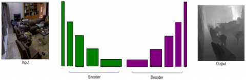
The architecture employed in this is based on the Encoder-Decoder concept. The encoder is used for feature extraction, and the decoder is used to improve the depth map's resolution. The deep learning model used for the encoder is EfficientNet-B0, a new model developed using a compound scaling approach. A decoder consisting of consecutive UpSampling blocks and convolutional and ReLu activation layers are added to upscale the image to the desired resolution. The name 'EfficientNet' emphasizes that this model is minimal in terms of the number of training parameters requirement and computational power. Yet, it delivers efficiencies more excellent than the previous state of the art deep learning models. In this project, the depth information is extracted in the form of a depth map. A depth map is an image that consists of RGBD parameters in which the D indicates the Depth. Many universities worldwide are working on this depth map estimation model and have brought out many databases. In this project, the NYU2 dataset (New York University) is used. It contains all images from various indoor scenes. The depth map estimation from these indoor scenes would help in the research study of indoor robot localization and movement.
As the NYU2 dataset contains both training images and corresponding depth labels, supervised deep learning techniques are employed for training the model. The transfer learning approach is used to ease computation. In this project, EfficientNet-B0 is used in the encoding and Bilinear UpSampling, Conv. and ReLu activation layers are included in the decoder architecture. DenseNet-121 and ResNet-50 architectures are also experimented with and compared with the EfficientNet-B0 model.
Contribution of the paper:
The prior works on the dense-depth estimation model and preliminaries are presented in section 2. The proposed methodology for depth estimation is proposed in section 3. Experimental results are discussed in section 4. Conclusions are provided in section 5.
The research on depth map estimation has a long history of 40 years. Generally, the Depth of the image is estimated by taking photographs of the same object at slightly different locations. Later disparity maps are drawn by taking the correspondence/similarity between the images. These disparity maps when scaled by focal lengths give the Depth of the field. Stereo vision is the motivation behind the Structure from Motion (SFM). It is proposed that by dividing the images [1] into groups and testing for rigid interpretation will result in the decomposition of scenes from motion. The structure has been used to map the 3D topography of the surface captured by Unmanned Aerial Vehicle [2]. The results obtained from SFM were comparable with those of Terrestrial Laser Scanning (TLS) surveys. ORB SLAM has been effectively proposed for 3D depth information [3]. Depth can be obtained from sparse features using SFM through structural similarities and other feature correspondences like texture variations, defocus, etc. The disparities of several 3D points are mapped to pixels of two images using the triangulation principle [4, 5].
The breakthrough in the monocular work was carried out by the researchers at Stanford University [6], in which they used a supervised learning approach for the depth estimation problem. Their supervised model used a discriminatively-trained Markov Random Field (MRF) that incorporates multiscale local and global image features and models both depths at individual points and the relation between depths of different points. Torralba and Oliva [7] integrated global image structure analysis and local features for depth map estimation from monocular images. Gabor wavelets were utilized for local feature extraction and the mean of the amplitude spectrum for capturing global features.
Guo et al. [8] demonstrated that haze could be used as a global feature to estimate the depth map from a single-view image. In another paper, a defocus map was used to estimate the depth map from a single image [9]. Considering the spatial layout, much more accurate depths were obtained [10]. 3D based object detector was developed using perspective cues from the global scene geometry. This detector is competitive with an image-based detector built using state-of-the-art methods; however, combining the two produces a notably improved detector because it unifies contextual and geometric information. A branch and bound approach was put forward, which splits the label space in terms of candidate sets of 3D layouts and efficiently bounds the potentials in these sets by restricting each face's contribution.
A compromise between the Spatial and Depth resolutions can improve network training [11]. Regression-classification Cascaded Network (RCNN) explicitly trains two separate networks, one which works on the problem of regression, i.e., generating low-resolution depth maps and at an individual scale in a continuous fashion. The other network poses this problem as a classification one and globally classifies different depth maps.
Monocular depth map estimation is an ill-posed problem. The depth estimation becomes complex with insufficient information in the images. Also, scale ambiguities, over/under illumination, and many more such image properties alleviate the complexity. Many machine learning and deep learning methodologies have tried to generate depth maps from monocular images with/without dataset. Machine learning and deep learning have paved the way for many advancements in the field of Computer vision. The pioneering research of CNN initially was propelled by the paper of LeCun et al. [12]. Gradient-based learning is introduced to synthesize a complex decision surface that can classify high-dimensional patterns. AlexNet started the revolution in Deep Learning in the year 2012 [13]. CNN is used for Image classification. AlexNet net won the 2012 ILSVRC (ImageNet Large-Scale Visual Recognition Challenge). Since then, many deep networks have developed, which further increased the efficiency of classification. The regression task involves comparing a relationship between one dependent variable and a series of independent variables. In one of the classic regression problems, the Depth map may change depending on the type of camera used. CAM-Convolution neural networks [14] are used to provide an ideal condition for their functioning. These convolutional layers take camera parameters like Calibration, focal length, etc.
A Depth map image using a Multiscale deep network is proposed by Fischer et al. [15] using two deep network stacks; one that makes a coarse global prediction based on the entire image and another that refines this prediction locally. They also applied a scale-invariant error to help measure depth relations rather than scale. The depth map may change depending on the type of camera used.
Camera Aware Multi-Scale-Convolutions [14] were employed in the encoder-decoder design. These convolutional layers take camera parameters like Calibration, focal length, etc. The first breakthrough was obtained by Eigen et al. [16] when they plotted a depth map image using a Multiscale deep network. They have used two deep network stacks; one that makes a coarse global prediction, and the other stack refines the local prediction. They also applied a scale-invariant error to measure depth relations rather than the scale.
Li et al. [17] removes the ambiguity for mapping images with Depth by combining pretrained RESNET with UpSampling blocks based on residual learning. Eigen and Fergus [18] proposed multiscale convolutional network architecture to apply three different computer vision tasks: Depth estimation, surface normal, and semantic labeling with slight modifications. The predictions of the depth map are improved by capturing image fine details with the sequence of scales. Depth map estimation is used in obstacle detection [19]. ResNet [20] is a very revolutionary architecture introduced in the deep learning arena. ResNet has also changed the retrieval efficiency of a depth map estimation problem. Residual learning is presented in the network to use layers with more Depth, which improves accuracy. Depth map estimation using residual networks has drastically increased the retrieval efficiency and decreased the computational power and memory requirement.
The usage of ResNet [21] improved the output resolution and accuracy of the overall model by training with just a few parameters. This model outperformed previous approaches to depth map estimation. Deep architectures and Residual networks were propelled with the pioneering work of using DenseNet architecture [22] in finding depth maps. DenseNet 169 was used to extract the features of the depth map using an encoder-decoder concept, in which the DenseNet layers form the feature extraction part and the UpSampling layers form the decoder part. In reconstructing the image, Bilinear UpSampling is used. Convolution layers alone with the UpSampling process is used rather than deconvolution and unpooling layers.
The upsurge in IoT and EDGE devices necessitated reducing no. of parameters, computational intensity, and the network's overall structure. Lightweight auto-encoder is proposed using MobileNet [23] also depthwise decomposition is used in both encoder and decoder architecture along with the pruning of the network. Mobilenet is gaining much significance in the field of deep learning. Large scale networks are pretrained on huge datasets—the network and its trained weights are employed in the depth regression problem. The pretrained network proposed by Alhashim and Wonka [22] is DenseNet-169. Supervised learning-based methods require a considerable amount of labeled datasets for training. Unsupervised techniques are used for alleviating the need for labeling in supervised models. One such approach estimated the depth map with left-right consistency methodology [24]. Disparity maps are generated by considering an image reconstruction loss. Training data is generated intrinsically by finding the correlations, correspondences between the different images of a dataset. Siamese and GAN networks are increasingly used in the self-supervised domain. GAN utilizes a Generator and a discriminatory network. A generator network generates random noise, and a discriminative network learns by comparing the network with sparse ground truth labels. GAN models have been used in-depth estimation. Siamese learning is also known as One-shot learning since only one training class is sufficient to train the network. A similarity function, which takes two variables (Images in our case), is solved by taking the single class label. This method was utilized for depth map estimation in robotic surgery [25]. The da Vinci surgical platform used in robotic surgery has the flexibility for allowing preoperative information to be incorporated into the live procedures using Augmented Reality (AR). Therefore scene depth estimation is essential in AR for 3D correspondence between the preoperative and intraoperative organ models. Scene depth estimation is a prerequisite for AR, as accurate registration requires 3D correspondences between preoperative and intraoperative organ models. The model consists of an autoencoder for Depthprediction and a differentiable spatial transformer for training the autoencoder on stereo image pairs without ground truth depths. The loss function in such adversarial networks relies on the loss function of joint correspondence of predicted depth values at the patch-level instead of pixel-level [26]. Unsupervised/self-supervised methodologies suffer from the problem of collapsing the network during training due to diverse datasets. The spectral normalization method was employed to avoid this problem. A technique using a Cyclic GAN was proposed [27]. Two generative networks are organized cyclically and later jointly trained with adversarial learning for reconstructing the disparity map. Unsupervised/Semi-supervised seems to be the future, but they are computationally very complex. Hence, the majority of the studies still concentrate on the supervised approach.
Depth estimation was performed on datasets like the NYU depth dataset [28] and the KITTI dataset [29]. These datasets provide many data-labels captured by Depth sensing equipment like Velodyne-laser camera and Kinect camera. These accurate data-labels help in the efficient building up of the models. Many efficient models were developed using these datasets in a supervised, unsupervised or semi-supervised fashion. The real challenge arises when these models are needed to deploy on IoT and EDGE platforms. Some deep learning models are highly computationally intensive and require huge memory for storage. Lightweight networks that result in less parameterization and high efficient output are required in-depth map estimation. One such network called EfficientNet [30] is implemented in this network. This network scales all dimensions of depth/width/resolution using a compound coefficient. The effectiveness of this method is demonstrated by scaling up MobileNets and ResNet. This method achieved a higher state of the art accuracy than previous ConvNets yet being a much smaller network. The large scale version EfficientNet-B7 is about 8.7x times smaller and 6.1x faster than the best previous state of the art networks. In this project, EfficientNet-B0 is experimented alongside ResetNet-50 and DenseNet-121. The proposed research computes the number of the parameters required in-depth estimation using EfficientNet-B0 by Encoder Decoder architecture is shown in Figure 1. Loss and Validation loss values are plotted for all the three networks DenseNet-121, ResNet-50 and EfficientNet-B0.
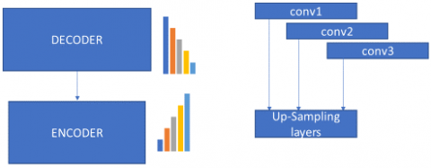
Figure 1. Encoder-decoder architecture
The proposed monocular depth estimation framework comprises EfficientNet-B0 combined with Bilinear UpSampling. The disadvantages in existing deep learning models motivated us to use the EfficientNet-B0. Generally, Deep learning models become computationally intensive and occupy more memory when the model 'depth, 'width' or 'resolution' increases. The arbitrary increasing of two or three of these parameters requires laborious manual tuning and still may give sub-optimal accuracy and efficiency. These three factors are scaled with constant ratio in the efficient net. If the resolution of the model increases, then the network requires more layers to escalate the receptive field and more channels to represent more fine-grained patterns on the High resolution image. The Depth in the network captures the higher level of abstractions in the image. The width of the model incorporated low-level features since more fine-grained patterns can be captured with more pixels. Hence, all three viz., Depth, width, and high resolution are required for adequate processing, but when all the three are combined, the network becomes very complicated. The compound scaling of depth/width and resolution was tried by Zoph et al. [31], and Real et al. [32]. This method suffers from manual intervention. An exceptional model with the name Efficient Net was developed by combining all the three parameters resulting in a significant increase in efficiency with a drastic decrease in the parameters. In the Efficient Net model, a compound scaling coefficient 'r' is utilized, which uniformly scales all the three parameters. Consider the following equations
Depth: $f=a^{r}$ (1)
Width: $d=b^{r}$ (2)
Resolution: $n=c^{\emptyset}$ (3)
where, $a \geq 1, b \geq 1, c \geq 1$ and $a \cdot b^{2} \cdot c^{2} \cong 2$, and a, b, c are scaling factors taken at small grid in the original tiny model. Generally, an increase in network complexity is determined by the rise in the number of FLOPS. In a conventional CNN, the number of FLOPS required is doubled if the network depth is doubled, but FLOPS are quadrupled if the network width or resolution is doubled. In this method the total increase of FLOPS is scaled by $\left(a \cdot b^{2} \cdot c^{2}\right)^{r}$, to curtail the number of flops required. From the above equation, the total FLOPS increase by $2^{r}$ approximately. EfficientNet follows the same fitting function as [33] i.e.,
$\operatorname{ACC}(m) \times[F L O P S(m) / T]^{w}$ (4)
The above fitting function is the optimization goal, where ACC(m) denotes the accuracy and FLOPS (m) represents the FLOPS of a model m, T is the target FLOPS, and w is the hyperparameter to balance accuracy and FLOPS. W is usually chosen as -0.07. Based on the above same search space [33], architecture similar to MnasNet called EfficientNet-B0 was developed. In terms of efficiency and requirement of the number of train parameters, EfficientNet-B0 outperformed much earlier state of the art methods. By scaling up the baseline network, different versions of the EfficientNet from B0 to B7 were obtained, where B7 being the highest scaled version among the EfficientNet. EfficientNet-B0 version is used in this project for the depth map estimation regression problem.
Deep Network only forms the Encoder part of our project. The Depth maps reconstructed must be the same dimension as the input. But the Deep Network reduces the spatial dimensions of the image. UpSampling is applied to increase the size of the depth image same as the size of the input image. Figure 2 depicts the UpSampling process for the given input image. For example, an image of 64 pixels of height and width, with 4096 pixels needs to be resized with the new pixel value of 256x256, i.e., 655356 pixels.
Following are the various types of interpolation methods used:
• Nearest neighbour: As the name suggests, the value is copied from the nearest pixel.
• Bilinear: Bilinear interpolation replaces each missing pixel with a linear interpolation of the nearest pixels.
• Bicubic: Here, the missing pixel is replaced with polynomial interpolation of neighboring pixels. It isn't easy to compute even when a smoother surface is produced.
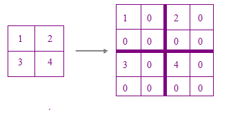
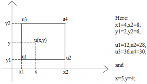
In this research, Bilinear UpSampling is utilized, which is the advancement of linear interpolation. In linear interpolation, interpolating any two variables is carried out on a rectangular grid. As the name indicates, bilinear deals with performing linear interpolation in two different directions. Although the operations carried out in each direction are linear, the entire output may not be linear; rather, it can be quadratic. The following provides an example of a Bilinear Up-Sampling operation.
Bilinear Up-sampling uses all the neighbouring pixels to calculate the value of an upsampled block. At first zeroes are padded as shown in Figure 2 and the weighted average of the two translated pixels are calculated for the output value. Bilinear interpolation produces smoother surface than linear interpolation and is less complicated than Bicubic interpolation. Similar operation is illustrated in the Figure 3. The UpSampling employed in this paper is a combination of Bilinear interpolation, convolution and ReLu layers. Deconvolutions is not used in this paper due to its high sensitivity to noise.
Figure 2. UpSampling process
Figure 3. Illustration of bilinear UpSampling operation
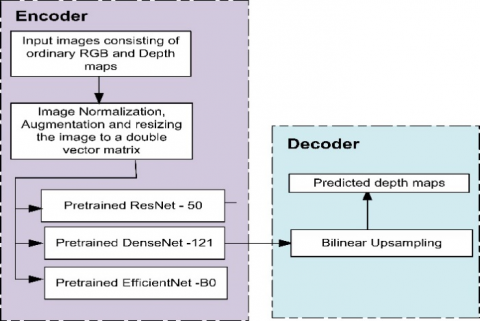
EfficientNet-B0 is used as an encoder in this project along with the bilinear-UpSampling method as the decoder. Experimentations were also conducted with ResNet and DenseNet architectures, and the results are compared with EfficientNet-B0. The Figure 4 illustrates the process flow.
Figure 4. Proposed depth estimation framework
Figure 5. Feature correspondence between Up-sampling and Encoder layers
Algorithmic steps for process flow:
|
Pseudo code for Encoder and Decoder design |
|
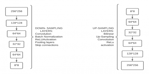
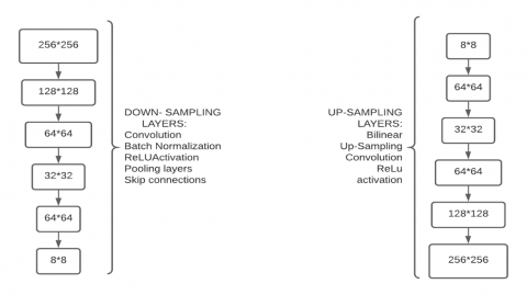
Inputs: Batch Normalization is performed to standardize the size of the input parameters of the network and to reduce the number of epochs; Input resolution is downsized from 640*480 to 256*256. Few data augmentation principles such as horizontal flipping, swapping color channels etc., but not rotation. Inpainting is done to color the depth maps. Test and Train set are passed for training the model. The input is then passed to encoder-decoder for depth reconstruction. Encoder: Input Resolution: 256*256, EfficientNet-B0 model The images of spatial resolution 256*256 in the database is encoded into 8*8 bits using Efficientnet -B0 as shown in Figure 6. Decoder: Input resolution: 8*8 The images of spatial resolution 8*8 produced in the encoder stage is decoded into 256*256 bits using Bilinear interpolation as shown in Figure 7. |
All the images in the dataset are of 640×480 size. All the images are downsized to 256×256, including the output predicted depth maps.
Figure 6. Encoding steps for proposed depth map estimation using EfficientNet-B0
Figure 7. Decoding steps for proposed depth map estimation using EfficientNet B0
This experimentation was initially executed on a local computer with an I5 processor (2.4Ghz processing speed) and 8GB of RAM. 90min was taken for 2 epochs experimentation. Google Colab Jupyter environment which consists of 12GB of VRAM is used to overcome the computational limitations. The average running time for 50 epochs on 5000 images was 5.5hrs. The zipped dataset is first loaded into Google Drive, and the drive is mounted on to the Colab notebook. Custom UpSampling layers, AutoAugmented custom object, and some other utilities are loaded before training. The total time taken for training the model is 6hrs.
Figure 8. Ground truth depth maps
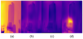
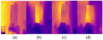
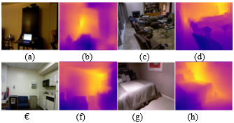
In the Experimentation two different datasets are used, the first database comprises of 500 heterogeneous images, out of which 400 are used for training and 100 for testing. The second database comprises of 5000 heterogeneous and homogeneous images, out of which 4400 are used for training and 600 images for testing. Ground truth and depth maps are presented in Figure 8. All the three models DenseNet-121, ResNet-50 and EfficientNet-B0 follow the model parameters as defined in Table 1. Figure 9 (a)-(d) illustrate the depth maps of the ground truth, ResNet-50, DenseNet-121 and EfficientNet-B0 respectively when experimented on the first dataset. Similarly, Figure 10 (a)-(d) illustrate the depth maps of the ground truth, ResNet-50, DenseNet-121 and EfficientNet-B0 respectively when experimented on the second dataset. Figure 11 (a), (c), € and (g) shows the original images of different scenes and Figure 11 (b), (d), (f) and (h) shows the corresponding depth map results obtained with the EfficientNet model. The results obtained from Figures 9 and 10 shows the effectiveness of EfficientNet when compared with the other two nets in terms of resolution.
Table 1. Model parameters and their corresponding values
|
Model Parameters |
Value |
|
Learning Rate |
0.0001 |
|
Optimizer |
Adam |
|
No.of Epochs |
50 |
|
Batch Size |
8 |
|
LossFunction |
Customized |
Figure 9. The different dense depth maps with 500 images (a) Ground Truth (b) ResNet-50 (c) DenseNet-121 (d) EfficientB0
Figure 10. The different dense depth maps with 5000 images (a) Ground Truth (b) ResNet-50 (c) DenseNet-121 (d) EfficientNet-B0
Figure 11. EfficientNet-B0 architecture with 5000 images experimentations (a)(c)(e)(g) and (b)(d)(f)(h) are the ground truth images and their depth maps with EfficientNet-B0
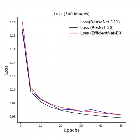
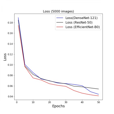
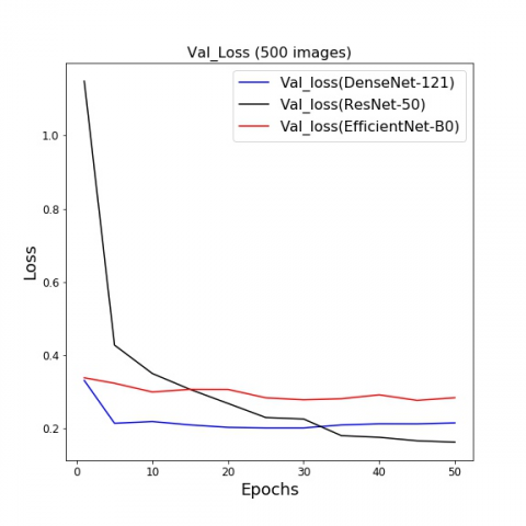
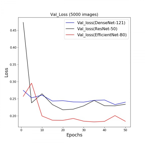
Plots are drawn for Loss values with respect to various epochs for the three models and are depicted in Figure 12 and Figure 13 for the first and second dataset respectively. Similarly, plots are drawn for Validation Loss values with respect to various epochs for the three models and are depicted in Figures 14 and 15 for the first and second dataset respectively. Tables 2 and 3 depict the Mean absolute Error (MAE) of the first and second datasets. From the Table 2, it is observed that Efficient Net has low MAE when compared with the other two nets. From Table 3 the MAE is low for ResNet-50. These results indicate that the EfficientNet-B0 outperforms the other two nets for depth estimation when heterogeneous or distinct images are used in the database. Besides this, EfficientNet-B0 outperforms in case of validation loss as shown in Figure 15. Jaccard Index is also a similarity coefficient that statistically measures the similarities between sample sets. Jaccard is defined as the ratio between the intersection size to the union size between two sample sets. F1 score is the harmonic mean of precision and recall known as the Dice similarity coefficient (DSC). It is a weighted average technique that evaluates the model extensively than the accuracy especially in regression problems. Table 4 shows the F1 score and Jaccard score values obtained for various models.
Overall a good trade-off between the size of the model and the efficiency can be obtained using EfficientNet-B0.
Figure 12. Plot depicting the loss for 500 images set
Figure 13. Plot depicting the loss for 5000 image experimentation
Figure 14. Validation loss plot for 500 images dataset
Figure 15. Validation loss plot for 5000 images
Table 2. Mean Absolute Error (MAR) comparison (500 images)
|
Epochs |
ResNet-50 |
DenseNet-121 |
EfficientNet-B0 |
|
1 |
1.1477 |
1.2060 |
1.0967 |
|
10 |
0.3506 |
0.3174 |
0.2675 |
|
20 |
0.2690 |
0.2226 |
0.1876 |
|
30 |
0.2266 |
0.2084 |
0.1385 |
|
40 |
0.1766 |
0.1626 |
0.1155 |
|
50 |
0.1633 |
0.1468 |
0.1012 |
Table 3. Mean Absolute Error (5000 images)
|
Epochs |
ResNet-50 |
DenseNet-121 |
EfficientNet-B0 |
|
1 |
0.9044 |
1.1477 |
1.0154 |
|
10 |
0.2215 |
0.3506 |
0.2351 |
|
20 |
0.1551 |
0.1633 |
0.1655 |
|
30 |
0.1256 |
0.1371 |
0.1412 |
|
40 |
0.1103 |
0.1219 |
0.1257 |
|
50 |
0.1012 |
0.1119 |
0.1139 |
Table 4. F1-score and Jaccard score comparison
|
Parameter/Neural-Net |
500 Images Dataset |
5000 Images Dataset |
||
|
F1-Score |
Jaccard Score |
F1-score |
Jaccard Score |
|
|
ResNet-50 |
0.54 |
0.64 |
0.65 |
0.68 |
|
DenseNet-121 |
0.58 |
0.65 |
0.66 |
0.69 |
|
EfficientNetB0 |
0.58 |
0.66 |
0.67 |
0.69 |
In this work, we propose a monocular depth estimation using encoder and decoder architecture. The encoder is a lightweight network EfficientNet-B0, and bilinear interpolation is used in the decoder to increase the model parameters. The results confirm that EfficientNet-B0 would be more efficient for high-resolution images, since the resolution scaling is one of the critical factors of the EfficientNet-B0. Further, due to varied scaling, it has also been observed that EfficientNet-B0 delivers low validation loss compared to other models when experimented on 5000 images. The rate of loss is less in EfficientNet-B0 compared with ResNet-50 and DenseNet-121 when the resolution of input is high.
In the future, the motto would be to develop a full-scale deployable model especially for autonomous cars. Datasets like KITTI which consists of outdoor scenes taken from a velodyne LIDAR camera installed on a car can serve such purposes. However, datasets may not be available for all the scenarios. The research will also concentrate on Semi-supervised and Unsupervised employing networks such as GAN and Siamese, which already have outstanding performance with meager labels. This knowledge needs to integrate into IoT and edge for robotic surgery, 3D scene analysis, and autonomous car systems.
[1] Zhang, C., Lin, Y., Zhu, L., Liu, A., Zhang, Z., Huang, F. (2019). CNN-VWII: An efficient approach for large-scale video retrieval by image queries. Pattern Recognition Letters, 123: 82-88. https://doi.org/10.1016/j.patrec.2019.03.015
[2] Ullman, S. (1979). The interpretation of structure from motion. Proceedings of the Royal Society of London. Series B. Biological Sciences, 203(1153): 405-426. https://doi.org/10.1098/rspb.1979.0006
[3] Mur-Artal, R., Montiel, J.M.M., Tardos, J.D. (2015). ORB-SLAM: A versatile and accurate monocular SLAM system. IEEE Transactions on Robotics, 31(5): 1147-1163. https://doi.org/10.1109/TRO.2015.2463671
[4] Zou, L., Li, Y. (2010). A method of stereo vision matching based on OpenCV. In 2010 International Conference on Audio, Language and Image Processing, Shanghai, China, pp. 185-190. https://doi.org/10.1109/ICALIP.2010.5684978
[5] Cao, Z.L., Yan, Z.H., Wang, H. (2015). Summary of binocular stereo vision matching technology. Journal of Chongqing University of Technology (Natural Science), 29(2): 70-75.
[6] Saxena, A., Chung, S.H., Ng, A.Y. (2006). Learning depth from single monocular images. Advances in Neural Information Processing Systems, pp. 1161-1168.
[7] Torralba, A., Oliva, A. (2002). Depth estimation from image structure. IEEE Transactions on Pattern Analysis and Machine Intelligence, 24(9): 1226-1238. https://doi.org/10.1109/TPAMI.2002.1033214
[8] Guo, F., Tang, J., Peng, H. (2015). Automatic 2D-to-3D image conversion based on depth map estimation. International Journal of Signal Processing, Image Processing and Pattern Recognition, 8(4): 99-112.
[9] Zhuo, S., Sim, T. (2011). Defocus map estimation from a single image. Pattern Recognition, 44(9): 1852-1858. https://doi.org/10.1016/j.patcog.2011.03.009
[10] Hedau, V., Hoiem, D., Forsyth, D. (2010). Thinking inside the box: Using appearance models and context based on room geometry. In European Conference on Computer Vision, Crete, Greece, pp. 224-237. https://doi.org/10.1007/978-3-642-15567-3_17
[11] Fu, H., Gong, M., Wang, C., Tao, D. (2017). A compromise principle in deep monocular depth estimation. arXiv preprint arXiv:1708.08267.
[12] LeCun, Y., Bottou, L., Bengio, Y., Haffner, P. (1998). Gradient-based learning applied to document recognition. Proceedings of the IEEE, 86(11): 2278-2324. https://doi.org/10.1109/5.726791
[13] Krizhevsky, A., Sutskever, I., Hinton, G.E. (2012). ImageNet classification with deep convolutional neural networks. Advances in Neural Information Processing Systems, pp. 1097-1105.
[14] Facil, J.M., Ummenhofer, B., Zhou, H., Montesano, L., Brox, T., Civera, J. (2019). CAM-Convs: Camera-aware multiscale convolutions for single-view Depth. In Proceedings of the IEEE Conference on Computer Vision and Pattern Recognition, Long Beach, CA, USA, pp. 11826-11835. https://doi.org/10.1109/CVPR.2019.01210
[15] Fischer, P., Dosovitskiy, A., Brox, T. (2015). Image orientation estimation with convolutional networks. German Conference on Pattern Recognition, Aachen, Germany, pp. 368-378. https://doi.org/10.1007/978-3-319-24947-6_30
[16] Eigen, D., Puhrsch, C., Fergus, R. (2014). Depth map prediction from a single image using a multiscale deep network. Advances in Neural Information Processing Systems, Montreal, Canada, pp. 2366-2374.
[17] Li, B., Shen, C., Dai, Y., Van Den Hengel, A., He, M. (2015). Depth and surface normal estimation from monocular images using regression on deep features and hierarchical CRFS. Proceedings of the IEEE Conference on Computer Vision and Pattern Recognition, pp. 1119-1127. http://dx.doi.org/10.1109%2FCVPR.2015.7298715
[18] Eigen, D., Fergus, R. (2015). Predicting depth, surface normals and semantic labels with a common multiscale convolutional architecture. Proceedings of the IEEE International Conference on Computer Vision, NW Washington, DC, United States, pp. 2650-2658. https://doi.org/10.1109/ICCV.2015.304
[19] He, K., Zhang, X., Ren, S., Sun, J. (2016). Deep residual learning for image recognition. Proceedings of the IEEE Conference on Computer Vision and Pattern Recognition, pp. 770-778. https://doi.org/10.1109/CVPR.2016.90
[20] Mancini, M., Costante, G., Valigi, P., Ciarfuglia, T.A. (2016). Fast robust monocular depth estimation for obstacle detection with fully convolutional networks. 2016 IEEE/RSJ International Conference on Intelligent Robots and Systems (IROS), Daejeon, Korea (South), pp. 4296-4303. https://doi.org/10.1109/IROS.2016.7759632
[21] Ma, X., Geng, Z., Bie, Z. (2017). Depth estimation from single image using CNN-residual network. SemanticScholar, 1-8.
[22] Alhashim, I., Wonka, P. (2018). High quality monocular depth estimation via transfer learning. arXiv preprint arXiv:1812.11941.
[23] Wofk, D., Ma, F., Yang, T.J., Karaman, S., Sze, V. (2019). Fastdepth: Fast monocular depth estimation on embedded systems. In 2019 International Conference on Robotics and Automation (ICRA), Montreal, QC, Canada, pp. 6101-6108. https://doi.org/10.1109/ICRA.2019.8794182
[24] Godard, C., Mac Aodha, O., Brostow, G.J. (2017). Unsupervised monocular depth estimation with left-right consistency. 2017 IEEE Conference on Computer Vision and Pattern Recognition (CVPR), Honolulu, HI, USA, pp. 6602-6611. https://doi.org/10.1109/CVPR.2017.699
[25] Ye, M., Johns, E., Handa, A., Zhang, L., Pratt, P., Yang, G.Z. (2017). Self-supervised Siamese learning on stereo image pairs for depth estimation in robotic surgery. arXiv preprint arXiv:1705.08260.
[26] Chen, R., Mahmood, F., Yuille, A., Durr, N.J. (2018). Rethinking monocular depth estimation with adversarial training. arXiv preprint arXiv:1808.07528.
[27] Pilzer, A., Xu, D., Puscas, M., Ricci, E., Sebe, N. (2018). Unsupervised adversarial depth estimation using cycled generative networks. 2018 International Conference on 3D Vision (3DV), Verona, Italy, pp. 587-595. https://doi.org/10.1109/3DV.2018.00073
[28] Silberman, N., Hoiem, D., Kohli, P., Fergus, R. (2012). Indoor segmentation and support inference from RGBD images. European Conference on Computer Vision, Florence, Italy, pp. 746-760. https://doi.org/10.1007/978-3-642-33715-4_54
[29] Geiger, A., Lenz, P., Stiller, C., Urtasun, R. (2013). Vision meets robotics: The KITTI dataset. The International Journal of Robotics Research, 32(11): 1231-1237. https://doi.org/10.1177%2F0278364913491297
[30] Tan, M., Le, Q.V. (2019). Efficientnet: Rethinking model scaling for convolutional neural networks. arXiv preprint arXiv: 1905.11946.
[31] Zoph, B., Vasudevan, V., Shlens, J., Le, Q.V. (2018). Learning transferable architectures for scalable image recognition. 2018 IEEE/CVF Conference on Computer Vision and Pattern Recognition, pp. 8697-8710. https://doi.org/10.1109/CVPR.2018.00907
[32] Real, E., Aggarwal, A., Huang, Y., Le, Q.V. (2019). Regularized evolution for image classifier architecture search. Proceedings of the AAAI Conference on Artificial Intelligence, 33(1). https://doi.org/10.1609/aaai.v33i01.33014780