Xiujuan Luo
© 2021 IIETA. This article is published by IIETA and is licensed under the CC BY 4.0 license (http://creativecommons.org/licenses/by/4.0/).
OPEN ACCESS
Currently, three-dimensional (3D) imaging has been successfully applied in medical health, movie viewing, games, and military. To make 3D images more pleasant to the eyes, the accurate judgement of image quality becomes the key step in content preparation, compression, and transmission in 3D imaging. However, there is not yet a satisfactory evaluation method that objectively assesses the quality of 3D images. To solve the problem, this paper explores the evaluation and optimization of 3D image quality based on convolutional neural network (CNN). Specifically, a 3D image quality evaluation model was constructed, and a 3D image quality evaluation algorithm was proposed based on global and local features. Next, the authors expounded on the preprocessing steps of salient regions in images, depicted the fusion process between global and local quality evaluations, and provided the way to process 3D image samples and acquire contrast-distorted images. The proposed algorithm was proved effective through experiments.
convolutional neural network (CNN), three-dimensional (3D) image, quality evaluation, quality optimization
Currently, three-dimensional (3D) imaging has been successfully applied in medical health, movie viewing, games, and military [1-6]. Compared with two-dimensional (2D) images and videos, 3D images and videos have a variety of detailed depth information, and provide viewers with an excellent visual experience [7-12]. The display effect of 3D images is mainly affected by the elements used to produce 3D contents, including brightness, chroma, contrast, saturation, and parallax [13-18]. To make 3D images more pleasant to the eyes, the accurate judgement of image quality becomes the key step in content preparation, compression, and transmission in 3D imaging [19-23].
In order to transmit 3D images, the bandwidth of the video signals should be doubled. Starting from visual perception and binocular stereography of humans, Wu and Hong [24] proposed a new subjective method to evaluate image compression quality, in accordance with the features of human binocular vision and the psychophysics of 3D fusion. The new method overcomes the constraint of subjective evaluation system on traditional subjective quality evaluation methods. Hachicha et al. [25] put forward an effective 3D quality evaluation method to measure the human perception of 3D images. The method can compute in the wavelet transform domain, and predict the quality of 3D images under statistical framework.
The traditional 3D image quality assurance measures only involve the error check between reference and distorted images. Jadhav et al. [26] developed a mean-edge structural similarity algorithm, and observed the performance of the algorithm. Based on the binocular human visual system, Zheng et al. [27] presented a simplified reference model for the evaluation of 3D image quality, which processes each 3D image by dividing it into a binocular fusion part and a binocular competition part, under the guidance of internal generation mechanism. The model achieved satisfactory coefficients related to subjective perception. Chetouani [28] created a novel metric for 3D full-reference image quality, based on cyclopean image (CI) computation and 2D fusion of image quality measurement (IQM). The experimental results demonstrate the effectiveness of this metric.
The existing objective evaluation methods of 3D images face two main problems: inability to assign scientific weights to the views of 3D images; poor evaluation effect on left and right views with different degrees of distortion. To solve the problems, it is necessary to fully consider the visual attention features of human eyes, and explore the evaluation and optimization of 3D image quality based on convolutional neural network (CNN). The main contents of this work are as follows: (1) setting up a 3D image quality evaluation model; (2) proposing a 3D image quality evaluation algorithm based on global and local features, and detailing the algorithm flow; (3) explaining the preprocessing steps of salient regions in images, as well as the fusion process between global and local quality evaluations; (4) providing the way to process 3D image samples and acquire contrast-distorted images. The proposed algorithm was proved effective through experiments.
The proposed artificial neural network (ANN) is based on neural unit calculation model, whose structure is shown in Figure 1. Let ai and fω,r(a) be the input and output of neural unit, respectively. Then, we have:
${{f}_{\omega ,r}}\left( a \right)=g\left( {{\omega }^{T}}a+r \right)=g\left( \sum\limits_{i=1}^{m}{{{\omega }_{i}}{{a}_{i}}+r} \right)$ (1)
Let ω, r, and g(.) be the weight, bias, and activation function of neural unit, respectively. The entire ANN consists of m layers, in which the input of the current layer is the output of the previous layer. Let ei(k) be the output of neuron i on layer k; ωij(k) be the connection weight between neuron j on layer k and neuron i on layer k+1; ai be the input of the ANN. Then, we have:
$\begin{align} & e_{1}^{\left( 2 \right)}=g\left( \omega _{11}^{\left( 1 \right)}a+\omega _{12}^{\left( 1 \right)}{{a}_{2}}+\omega _{13}^{\left( 1 \right)}{{a}_{3}}+r_{1}^{\left( 1 \right)} \right) \\ & e_{2}^{\left( 2 \right)}=g\left( \omega _{21}^{\left( 1 \right)}{{a}_{1}}+\omega _{22}^{\left( 1 \right)}{{a}_{2}}+\omega _{23}^{\left( 1 \right)}{{a}_{3}}+r_{2}^{\left( 1 \right)} \right) \\ & e_{3}^{\left( 2 \right)}=g\left( \omega _{31}^{\left( 1 \right)}{{a}_{1}}+\omega _{32}^{\left( 1 \right)}{{a}_{2}}+\omega _{33}^{\left( 1 \right)}{{a}_{3}}+r_{3}^{\left( 1 \right)} \right) \\ & {{f}_{\omega ,r}}\left( a \right)=e_{1}^{\left( 3 \right)}=g\left( \omega _{11}^{\left( 1 \right)}e_{1}^{\left( 2 \right)}+\omega _{12}^{\left( 1 \right)}e_{2}^{\left( 2 \right)}+\omega _{13}^{\left( 1 \right)}e_{3}^{\left( 2 \right)}+r_{1}^{\left( 2 \right)} \right) \\\end{align}$ (2)
Suppose the weighted summation of all the inputs of neuron i on layer c equals ci(k). Then, the forward propagation of the ANN obeys:
$\begin{align} & c_{i}^{\left( 2 \right)}=\sum\nolimits_{j=1}^{m}{\omega _{ij}^{\left( 1 \right)}{{a}_{j}}+r_{i}^{\left( 1 \right)}} \\ & e_{i}^{\left( l \right)}=g\left( c_{i}^{\left( l \right)} \right) \\\end{align}$ (3)
A single-layer neural network cannot solve nonlinear tasks. To solve the problem, the proposed ANN maps each sample to the other space via nonlinear activation functions and hidden layer(s). The activation functions are initialized as sigmoid and tanh:
$g\left( c \right)=sigmoid\left( c \right)=\frac{1}{1+{{e}^{-c}}}$ (4)
$g\left( c \right)=tanh\left( c \right)=\frac{{{e}^{c}}-{{e}^{-c}}}{{{e}^{c}}+{{e}^{-c}}}$ (5)
For a given 3D image training data (a, b), the ANN loss function value obtained through forward propagation is denoted as Loss (ω, r). During error backpropagation, the neural residual of the last output layer can be calculated by:
${{\xi }^{K}}=\frac{\partial Loss\left( \omega ,r \right)}{\partial {{c}^{K}}}=\frac{\partial Loss\left( \omega ,r \right)}{\partial {{e}^{K}}}\oplus g'\left( {{c}^{K}} \right)$ (6)
The residual of layer k can be derived from the residual ξk+ 1 of layer k+1:
${{\xi }^{k}}={{\xi }^{k+1}}\frac{\partial {{c}^{k+1}}}{\partial {{c}^{k}}}={{\left( {{\omega }^{k}} \right)}^{T}}{{\xi }^{k+1}}\oplus g'\left( c_{i}^{k} \right)$ (7)
Based on the calculated residual, the partial derivatives of the ANN’s connection weight and bias can be calculated by:
$\frac{\partial Loss\left( \omega ,r \right)}{\partial {{\omega }^{k}}}=\frac{\partial Loss\left( \omega ,r \right)}{\partial {{c}^{k+1}}}\frac{\partial {{c}^{k+1}}}{\partial {{\omega }^{k}}}={{\xi }^{k+1}}{{\left( {{e}^{k}} \right)}^{T}}$ (8)
$\frac{\partial Loss\left( \omega ,r \right)}{\partial {{r}^{k}}}=\frac{\partial Loss\left( \omega ,r \right)}{\partial {{c}^{k+1}}}\frac{\partial {{c}^{k+1}}}{\partial {{r}^{k}}}={{\xi }^{k+1}}$ (9)
After solving the above two partial derivatives of each layer, the network parameters can be updated through gradient descent. During ANN training, the learning rate α determines the magnitude of each parameter update. Then, we have:
$\left\{ \begin{matrix} {{\omega }^{k}}\leftarrow {{\omega }^{k}}-\alpha \frac{\partial Loss\left( \omega ,r \right)}{\partial {{\omega }^{k}}} \\ {{r}^{k}}\leftarrow {{r}^{k}}-\alpha \frac{\partial Loss\left( \omega ,r \right)}{\partial {{r}^{k}}} \\\end{matrix} \right.$ (10)
To enhance the learning ability of ANN-based 3D image quality evaluation model, this paper locally normalizes the image samples for training. Firstly, the mean gray value and variance of 3D image pixels in the normalization region were solved. Then, the difference between the gray value of a pixel and the mean gray value was divided by variance. On a 3D image, the processing result of pixel (i, j) can be described by P(i, j). Let D be the constant to prevent division by zero; S and T be the size of the normalization region. Then, P(i, j) can be calculated by:
$\hat{P}\left( i,j \right)=\frac{P\left( i,j \right)-\lambda \left( i,j \right)}{\varepsilon \left( i,j \right)+D}$ (11)
where,
$\lambda \left( i,j \right)=\frac{1}{2S\times 2T}\sum\limits_{s=-S}^{s=S}{\sum\limits_{t=-T}^{t=T}{P\left( i+s,j+t \right)}}$. (12)
$\varepsilon \left( i,j \right)=\sqrt{\frac{1}{2S\times 2T}\sum\limits_{s=-S}^{s=S}{\sum\limits_{t=-T}^{t=T}{{{\left( P\left( i,j \right)-\lambda \left( i,j \right) \right)}^{2}}}}}$ (13)
Figure 1. Structure of a neural unit
Table 1. Overall structure of the proposed CNN model
|
Left view input |
32 kernels (9×9, 7×7, 5×5) |
Max pooling (3×3, 3×3, 3×3) |
50 kernels (7×7, 5×5, 3×3) |
Max pooling (3×3, 3×3, 3×3) |
100 kernels (7×7, 5×5, 3×3) |
Spatial pyramid (5, 5, 5) |
Fully-connected layer + dropout |
Fully-connected layer (300) |
Fully-connected layer (1) |
|
Right view input |
50 kernels (9×9, 7×7, 5×5) |
Max pooling (3×3, 3×3, 3×3) |
50 kernels (7×7, 5×5, 3×3) |
Max pooling (3×3, 3×3, 3×3) |
100 kernels (7×7, 5×5, 3×3) |
Spatial pyramid (5, 5, 5) |
The proposed CNN with multi-channel parallel inputs (CNN-G) was trained through stochastic gradient descent. Table 1 shows the structural parameters of the network. During the training, a batch of samples was trained in each iteration to effectively improve the training accuracy of our model. Let {ikm, iwm} be a distorted image for network training; zm be the subjective evaluation of human eyes; gh{ikm, iwm}; ω, r be the objective quality of 3D images outputted by CNN-G; Loss(ω) be the training error between network prediction and subjective quality evaluation of 3D images; η(ω) be the regularization term to suppress overfitting, which is positively proportional to network scale; μ be the weight attenuation parameter that suppresses the influence of the regularization term. Then, Loss(ω) can be expressed as:
$Loss\left( \omega \right)=\frac{1}{2M}{{\sum\limits_{m=1}^{M}{\left\| {{g}_{h}}\left( \left\{ {{i}_{km}},{{i}_{wm}} \right\};\omega ,r \right)-{{z}_{m}} \right\|}}^{2}}+\mu \eta \left( \omega \right)$ (14)
The momentum optimization method was adopted to update network parameters. Let ▽TE(ωτ) be the gradient of training loss function; τ be the number of training iterations; Uτ+1 be the weight update in iteration τ+1; ωτ+1 be the weight of iteration τ+1; λ be the momentum characterizing the weight update of the previous iteration on this iteration. Then, the weight update process can be described by:
${{U}_{\tau +1}}=\lambda {{U}_{\tau }}-\alpha \nabla Loss\left( {{\omega }_{\tau }} \right)$ (15)
${{\omega }_{\tau +1}}={{\omega }_{\tau }}+{{U}_{\tau +1}}$ (16)
When viewing an image, the human visual system focuses on the most interesting and salient area, that is, the human eyes pay uneven attention to different parts of the image. A 3D image is equivalent to a 2D image added with depth information. The human visual system cannot match all feature edges in a short time. Therefore, the quality of the entire 3D image can be measured by the quality of the 3D saliency map. This would improve the accuracy of quality prediction, and, to a certain extent, lower computing complexity. The quality of a 3D image is jointly affected by its parallax feature and spatial frequency. Hence, 3D saliency map can be obtained based on the parallax between 2D saliency map and 3D image.
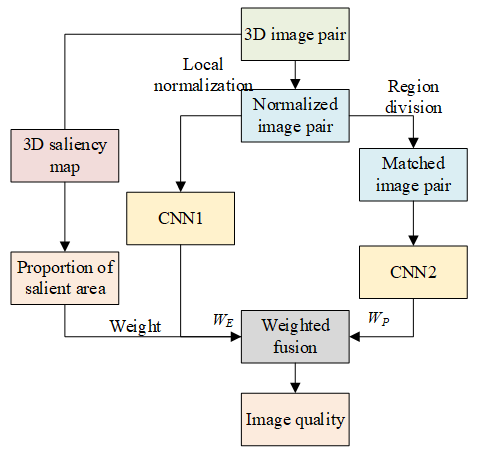
Figure 2 shows the flow of the proposed 3D image quality evaluation algorithm, which is based on global and local features. After local normalization, CNN 2 was adopted to comprehensively consider the influence of distortion on the whole 3D image, and to obtain the objective score of the overall quality of the 3D image. Then, the normalized 3D image was segmented into small blocks. These blocks were imported to CNN1 to comprehensively consider the influence of distortion on local details of the image, and to obtain the objective score of the local quality of the 3D image. Based on the saliency test on 3D image, the proportion of ultra-salient region in the saliency map was calculated, and taken as the weight to fuse the global and local scores of the 3D image into the final quality evaluation.
In the previous section, CNN2 is constructed from the angle of perceiving the overall information of the 3D image. Because the number of samples is too small for the training model, the model training is not sufficient. To solve the problem, local details should be extracted from the 3D image, and an independent model was constructed to evaluate the local quality of that image. Figure 3 presents the structure of the objective quality evaluation model for local areas of 3D images.
Figure 2. Framework of non-reference 3D image quality evaluation algorithm based on global and local image features
Figure 3. Structure of the objective quality evaluation model for local areas of 3D images
3.1 Preprocessing of salient areas
Let GSRE (a, b) be the 2D saliency map of the right view of most people; PARE (a, b) be the parallax map with the right view as the benchmark; LT (a, b) be the 3D saliency map. This paper firstly compute GSRE(a, b) with image-based visual saliency algorithm, and then obtains PARE(a, b) through rapid 3D matching. Finally, the saliency map and right view parallax map were linearly weighted to obtain LT (a, b), using the weights ω1 and ω2, respectively. Then, LT (a, b) can be calculated by:
$LT\left( a,b \right)={{\omega }_{1}}P{{A}_{F}}\left( a,b \right)+{{\omega }_{2}}G{{S}_{F}}\left( a,b \right)$ (17)
where, ω1 and ω2 add up to 1.
Based on fuzzy mathematics, this paper describes and optimizes the features of 3D saliency map, and further obtains the corresponding binary mask image N. If a pixel in the 3D image belongs to the saliency area, then the pixel value is 1; otherwise, the pixel value is 0. The description and optimization processes are detailed as follows:
Suppose the 3D saliency map is characterized by the discourse domain A. The pixels a can be divided into a salient area E and a non-salient area R:
$E\cup R=A\text{ }E\cap R=\varphi $ (18)
In the original 3D mage, the membership of a pixel to the salient area can be measured by the gray value of the saliency map. Then, the membership of pixel a to E can be calculated by:
$E\left( a \right)=\frac{a}{255}$ (19)
The final goal of preprocessing the salient area in the 3D image is to obtain E. Therefore, the image needs defuzzification. Let ψ be the segmentation threshold determined by the maximum between-class variance method. Then, a mask image N can be obtained through threshold segmentation:
$N\left( a \right)=\left\{ \begin{align} & 1\text{ }E\left( a \right)>\psi \\ & 0\text{ }Otherwise \\\end{align} \right.$ (20)
If E(a) is greater than ψ, then a belongs to the salient area of the 3D image, and corresponds to the white area in N; otherwise, a does not belong to the salient area of the 3D image, and corresponds to the black area in N.
The saliency of 3D image was tested in three steps with a bottom-up saliency testing algorithm:
Step 1. The local control kernel (LCK) is adopted to analyze the difference between pixel values in the original image, and further derive the local structural information, kernel size, and kernel shape. The LCK function can be described as:
$LCK\left( {{a}_{\tau }}-{{a}_{i}} \right)=\frac{\sqrt{det\left( co{{v}_{k}} \right)}}{{{\gamma }^{2}}}{{e}^{\frac{{{\left( {{a}_{\tau }}-{{a}_{i}} \right)}^{T}}co{{v}_{\tau }}\left( {{a}_{\tau }}-{{a}_{i}} \right)}{-2{{\gamma }^{2}}}}},co{{v}_{k}}\in {{\Re }^{2\times 2}}$ (21)
Let k (k =1,…, t2) be a pixel in the image; covk be the covariance matrix of the gradient vector of the pixel; ak =[al, a2]T be the spatial coordinates of the pixel; γ be the global smoothing parameter.
Step 2. The LCK obtained in Step 1 is normalized, and the result is taken as a feature to build a feature matrix Gi. Then, the similarity between Gi and the feature matrix Gj of an adjacent pixel is compared.
Step 3. Let MAi be the saliency of a pixel; σ be the function of cosine similarity between matrices. The saliency of the pixel can be derived from the similarity between Gi and Gj:
$M{{A}_{i}}=\frac{1}{\sum\nolimits_{j=1}^{M}{exp\left( \frac{-1+\sigma \left( {{G}_{i}},{{G}_{j}} \right)}{{{\varepsilon }^{2}}} \right)}}$ (22)
The saliency map of the 3D image can be plotted based on the calculated MAi value.
3.2 Fusion between global and local quality evaluations
The objective quality of 3D image can be evaluated from the angle of perceiving the information of the overall semantics and local details. The final quality score must comprehensively reflect the global and local evaluations. The two evaluations need to undergo weighted fusion:
$QE={{\delta }_{LT}}{{W}_{E}}+\left( 1-{{\delta }_{LT}} \right){{W}_{P}}$ (23)
Let QE be the final quality evaluation of the 3D image; WE and WP be the global and local evaluations, respectively; Ω be the ultra-salient area in the image. The mean saliency of the entire 3D image is smaller than the saliency of a pixel in Ω. In addition, the area of the entire image and the total number of pixels are denoted as MJ and NSI, respectively; the saliency of pixel (i, j) is denoted as MJ (i, j). Then, the proportion δLT of the salient area can be calculated by:
${{\delta }_{LT}}=\frac{\Omega }{MJ},\Omega =\left[ \left( i,j \right)|M{{J}_{k}}\left( i,j \right)\ge {{\overline{MJ}}_{k}},M{{J}_{s}}\left( i,j \right)\ge \overline{M{{J}_{s}}} \right]$ (24)
$\overline{MJ}=\Psi \left( MJ \right)=\frac{1}{N}\sum{\sum{_{\left( i,j \right)\in MJ}}}MJ\left( i,j \right)$ (25)
4.1 3D image processing
The influence of disturbances on quality evaluation should be eliminated to ensure the generality and representatives of the subjective evaluation of 3D image quality. This paper adopts the Grubbs’ test for outliers and the recommended method of BT.500 – ITU to clean out abnormal samples, and remove all their scores.
In the Grubbs’ test, the MP subjective scores of the 3D image are denoted as vi. The mean and standard deviation of all evaluations can be respectively calculated by:
$\overline{v}=\frac{\sum\limits_{i=1}^{{{M}_{P}}}{{{v}_{i}}}}{{{M}_{P}}}$ (26)
$MJ=\sqrt{\frac{\sum\nolimits_{i=1}^{{{M}_{P}}}{{{\left( {{v}_{i}}-\overline{v} \right)}^{2}}}}{{{M}_{P}}-1}}$ (27)
The Grubb’s value of each subjective evaluation can be calculated by:
${{H}_{i}}=\frac{\left| V-{{\overline{v}}_{i}} \right|}{MJ}$ (28)
To determine the confidence interval for subjective evaluations of image quality, the critical value of each subjective evaluation was looked up for in the Gurbb’s table. The suspicious value under a confidence can be defined as a Grubb’s value greater than the critical value.
To eliminate abnormal 3D image samples, the recommended method of BT.500 – ITU first calculates the mean and standard deviation of the scores of MP 3D images, yielding an N-dimensional mean vector and standard deviation vector. Then, the θ of the target 3D image can be calculated by:
${{n}_{v}}=\frac{\sum\limits_{i=1}^{{{M}_{P}}}{{{\left( {{v}_{i}}-\overline{v} \right)}^{v}}}}{{{M}_{P}}}$ (29)
$\theta =\frac{{{n}_{4}}}{{{\left( {{n}_{2}} \right)}^{2}}}$ (30)
If the scores of 3D images obey normal distribution, then the θ value belongs to [2, 4]; otherwise, the θ value does not belong to [2, 4]. If the scores of 3D image j obey normal distribution, then the critical value CVj of the image can be calculated by formula (31); otherwise, critical value CVj can be calculated by formula (32):
$C{{V}_{j}}=\overline{v}+2MJ$ (31)
$C{{V}_{j}}=\overline{v}+2\sqrt{5}MJ$ (32)
Two counters Xi and Yi were set up for target 3D image i. If the score is greater than the critical value CVj, then add 1 to Xi; otherwise, add 1 to Yi. If Xi and Yi satisfy the following inequality, then eliminate 3D image i:
${{X}_{i}}+{{Y}_{i}}>0.05\text{ }and\text{ }\frac{{{X}_{i}}-{{Y}_{i}}}{{{X}_{i}}+{{Y}_{i}}}<0.3$ (33)
The above two stages of filtering effectively prevent the quality evaluation being affected by disturbances, ensuring the accuracy of the final quality evaluation. The final evaluation of a 3D image is the statistical mean of the filtered evaluations. The statistical mean can be calculated by:
$F{{S}^{*}}=\sum\nolimits_{l=1}^{5}{{{m}_{l}}F{{S}_{l}}}/\sum\nolimits_{l=1}^{5}{{{m}_{l}}}$ (34)
Suppose there are 5 levels of 3D image quality. Let mq be the number of evaluations indicating that the image belongs to level q (q=1, 2, …, 5); FSq be the score of the 3D image belonging to level q. A good quality 3D image should at least receive 4 points. Hence, qualified 3D images must have an FS*≥4.
4.2 Acquisition of contrast-distorted images
This paper calculates the contrast of the saliency map of the original 3D image, using the 4-nearest neighbors algorithm. Based on the calculated contrast, the contrast distortion of the left and right views of the original image was obtained through linear contrast transform, yielding the contrast-distorted 3D image pair to be evaluated.
Let (i, j) be the coordinates of the central black pixel; (i, j-1), (i, j+1), (i-1, j), and (i+1, j) be the coordinates of the upper, lower, left, and right gray pixels, i.e., the 4-nearest pixels (i*, j*).
Taking pixel block w×h for example, the gray value of pixel (i, j) is denoted as HD(i, j), and the gray values of the 4-nearest pixels are denoted as HD(i’, j’), ξ[(i, j), (i’, j’)]=[HD(i, j)-HD(i’, j’)]. The probability for the gray difference between adjacent pixels be ξ is denoted as DPξ[(i, j), (i’, j’)]. Then, the contrasts of the 4-nearest neighbors of the entire image can be calculated by:
$FNNC=\sum\limits_{i=1}^{w}{\sum\limits_{j=1}^{h}{{{\left( \xi \left[ \left( i,j \right),\left( i',j' \right) \right] \right)}^{2}}}}H{{D}_{\xi }}\left. \left[ \left( i,j \right),\left( i',j' \right) \right] \right)$ (35)
During the contrast transform of the image, the mean gray value is denoted as PJ, the contrast adjustment factor as χ∈[1, 1], and the gray value of the input pixel as GVH. Then, the gray value GVV of the pixel after contrast transform can be calculated by:
$G{{V}_{V}}=PJ+\left( G{{V}_{H}}-PJ \right)\times \left( 1-\chi \right)$ (36)
If the contrast of the 3D image increases, then χ>0, and the slope of the corresponding line is greater than 1; if the contrast of that image decreases, then χ<0, and the slope of that line is smaller than 1. Through the contrast transform, the image contrast will remain the same if the mean brightness does not change. In this case, χ equals zero.
Due to the difference of 3D images in original contrast, the normalized contrast was defined as the ratio of the original contrast to the linearly transformed contrast. The least squares piecewise linear fitting was adopted to process two sets of 3D image samples. The fitting results on the two sample sets, i.e., similarity and difference of normalized contrasts, are shown in Figures 4 and 5, respectively. As shown in Figure 4, the 3D images with good quality evaluation correspond to the area enclosed by the broken lines. As shown in Figure 5, the 3D images with different quality evaluations correspond to different normalized contrast errors between left and right views. The error is characterized by the area enclosed by the broken lines. If a 3D image is of high quality, then the normalized contrast error between left and right views is positive; if a 3D image is of poor quality, then the said error is negative.
Traditionally, 3D image quality evaluation directly quantifies the influence of the contrast of the whole image over image quality, without fully considering visual saliency. Figure 6 compares the experimental results of the reference model (the area enclosed by blue broken lines) and our model (the area enclosed by red broken lines).
Judging by the overlapping areas between the results of the two models, the areas obtained by our model were basically contained in those obtained by the reference model. Hence, the quality evaluation of salient area is strongly consistent with that of entire image, which agrees with the theoretical situation.
Figure 4. Similarity of normalized contrasts of 3D images
Figure 5. Difference of normalized contrasts of 3D images
Figure 6. Experimental results of reference model and our model
From the areas obtained by reference model but not by our model, it can be learned that, when the normalized contrast was low in the left view, the right view of the regions obtained by the reference model was also low. But the two views had low brightness and fuzzy textures, who do not adapt to the visual properties of the human eyes. By contrast, in the areas obtained by our model, when the normalized contrast was low in the left view, the normalized contrast in the right view was much higher than that value, making up for the defect brought by the excessively small left view contrast. To sum up, the areas obtained by our model are more in line with our visual properties than those obtained by the reference model. Following our model, the high-quality 3D images fall in a visually comfortable range.
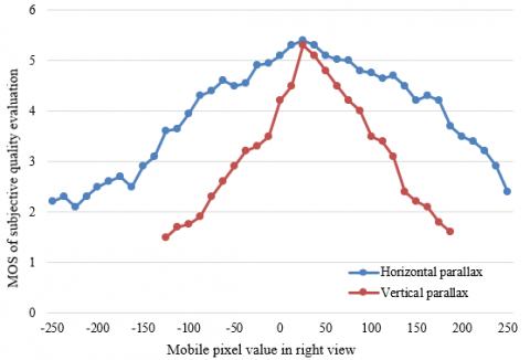
Figure 7. Relationship between MOS of subjective quality evaluation and horizontal parallax
This paper processes the MOS of subjective quality evaluation and experimental results on horizontal parallax, through least squares piecewise linear fitting. Figure 7 presents the relationship curve between the two values. With the variation in horizontal parallax, the statistical average of the MOS of subjective quality evaluation was solved for multiple 3D images, and the fitted lines are shown in Figure 7.
Table 2. Properties in different regions
|
|
Region Ⅰ |
Region Ⅱ |
Region Ⅲ |
Region Ⅳ |
Region Ⅴ |
|
Depth |
In-screen |
Out-of-screen |
Out-of-screen |
Out-of-screen |
Out-of-screen |
|
Parallax |
0~26 |
26~86 |
>86 |
0~-55 |
<-55 |
|
MOS range |
4.7~4.8 |
4.7~4 |
<4 |
4.5~4 |
<4 |
|
Qualified? (Yes/No) |
Yes |
Yes |
No |
Yes |
Yes |
The five regions in Figure 7 were numbered I-V in turn. The 3D images with MOS>4 were deemed as meeting quality requirements. Table 2 presents the attributes of different areas. Specifically, Region I, where the subjective evaluation increases, is the strongly good area, with a parallax of 0-25 pixels. In the region, if the parallax continues to increase, the 3D image becomes more and more stereo, and the subjective evaluation increases till reaching the peak. Region II, where the subjective evaluation decreases, is the slightly good area, with a parallax of 25-85 pixels. In the region, the visual experience increases with positive parallax, but MOS decreases with the growing positive parallax. Region IV, where the subjective evaluation decreases, is the good area, with a parallax of 0-50 pixels. In the region, the 3D image can be viewed well with each eye, creating a vivid visual experience. Overall, the above three regions offer a good stereo sense, and lower the visual fatigue of viewers. Regions III and V, where the subjective evaluation decreases, are both poor areas. The parallax range of Region V surpasses 50 pixels, while that of Region III exceeds 85 pixels. In these two regions, further growth of parallax easily leads to an excessively large angle between out-of-screen line-of-sights, making viewers dizzy or puffy in the eyes.
Figure 8 compares the MOS trends under different horizontal parallaxes and vertical parallaxes. The MOS curve of horizontal parallax descended deeper than that of vertical parallax. When the MOS of subjective quality evaluation dropped to 2, the horizontal and vertical parallaxes were 230 and 80 pixels, respectively. From the quantification angle, the results confirm that the human eyes are more sensitive to vertical parallax than horizontal parallax.
Figure 8. MOS trends under different horizontal parallaxes and vertical parallaxes
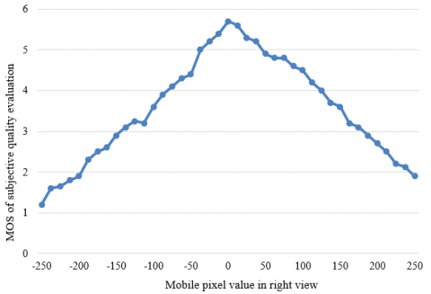
Figure 9. Experimental results on horizontal parallax distortion of reference model
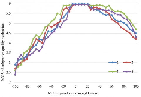
To further verify the effectiveness of our model on 3D image quality evaluation, this paper designs a comparative experiment between our model and the evaluation model without visual attention mechanism. Based on the parallax range corresponding to good areas, the other parallax-distorted 3D images were subjected to quality evaluation. Figures 9 and 10 present the MOS trends of the reference model and our model under different horizontal parallaxes. It can be seen that, the MOS curve of the reference model did not rise in the range of positive parallax. Meanwhile, the MOS curve of our model had a small increasing interval. That is, the visual experience of 3D images with growing background parallax is better than that of zero-parallax images. The results confirm that the parallax range corresponding to good areas, which is obtained in this paper, match the visual features of the human eyes excellently. In addition, the MOS of the reference model almost did not change, when the parallax distortion was very small. By contrast, the MOS curve of our model changed greatly. This means the fusion between global and local quality evaluations helps the viewers perceive the small parallax distortion in the 3D image sensitively, which effectively pushes up experimental accuracy.
Figure 10. Experimental results on horizontal parallax distortion of our model
This paper presents a CNN-based evaluation and optimization of 3D image quality. After setting up a 3D image quality evaluation model, the authors developed the 3D image evaluation algorithm based on global and local features, explained the preprocessing of the salient area and the fusion between global and local quality evaluations, and presented the way to process 3D image samples and contrast-distorted images. Through experiments, the similarity and difference of normalized contrasts of 3D images were plotted, and the experimental results of the reference model were compared with those of our model, revealing that areas obtained by our model are more in line with the visual properties of the human eyes than those obtained by the reference model. Next, this paper processes the MOS of subjective quality evaluation and experimental results on horizontal parallax, through least squares piecewise linear fitting. The MOS trends of our model under different horizontal parallaxes were compared with those of the reference model. It can be seen that the MOS curve of our model changed relatively significantly, which further confirms the effectiveness of our model in 3D image quality evaluation.
[1] Liu, J., Xu, X., Liu, Y., Rao, Z., Smith, M. L., Jin, L., Li, B. (2021). Quantitative potato tuber phenotyping by 3D imaging. Biosystems Engineering, 210: 48-59. https://doi.org/10.1016/j.biosystemseng.2021.08.001
[2] Czarske, J.W., Scharf, E., Kuschmierz, R. (2019). Ultrathin lensless fiber endoscope with in situ calibration for 3D imaging. In Bio-Optics: Design and Application, DM2B-5. https://doi.org/10.1364/BODA.2019.DM2B.5
[3] Nagata, Y., Obara, M., Ihara, M., Yoshimori, K. (2019). 3D spectral imaging of fluorescent micro beads using multispectral incoherent holography. In Digital Holography and Three-Dimensional Imaging, W3A-9. https://doi.org/10.1364/DH.2019.W3A.9
[4] Thompson, A., Livina, V., Harris, P., Mohamed, I., & Dudley, R. (2019). Model-based algorithms for phenotyping from 3D imaging of dense wheat crops. In 2019 IEEE International Workshop on Metrology for Agriculture and Forestry (MetroAgriFor), 95-99. https://doi.org/10.1109/MetroAgriFor.2019.8909214
[5] Birla, M., Zou, J., Afkhami, Z., Duan, X., Li, H., Wang, T. D., Oldham, K. R. (2021). Multi-photon 3D imaging with an electrothermal actuator with low thermal and inertial mass. Sensors and Actuators A: Physical, 329: 112791. https://doi.org/10.1016/j.sna.2021.112791
[6] Nicolaescu, R., Rogers, C., Piggott, A.Y., Thomson, D.J., Opris, I.E., Fortune, S.A., Reed, G.T. (2021). 3D imaging via silicon-photonics-based LIDAR. In Silicon Photonics XVI, 11691: 116910G. https://doi.org/10.1117/12.2591284
[7] Hussain, M.M., Guo, H., Banerjee, P.P. (2021). Ptychographic coherent diffractive imaging, digital holography and structured light techniques for topographical 3D imaging. International Society for Optics and Photonics, In Pattern Recognition and Tracking XXXII, 11735: 117350H. https://doi.org/10.1117/12.2591274
[8] Tan, S., Yang, F., Boominathan, V., Veeraraghavan, A., Naik, G.V. (2021). 3D Imaging Using Extreme Dispersion in Optical Metasurfaces. ACS Photonics, 8(5): 1421-1429. https://pubs.acs.org/doi/10.1021/acsphotonics.1c00110
[9] Nitka, A. (2019). The use of 3D imaging to determine the orientation and location of the object based on the CAD model. In Photonics Applications in Astronomy, Communications, Industry, and High-Energy Physics Experiments 2019. International Society for Optics and Photonics, 11176: 111760Z. https://doi.org/10.1117/12.2536895
[10] Mhaske, P., Condict, L., Dokouhaki, M., Katopo, L., Kasapis, S. (2019). Quantitative analysis of the phase volume of agarose-canola oil gels in comparison to blending law predictions using 3D imaging based on confocal laser scanning microscopy. Food Research International, 125: 108529. https://doi.org/10.1016/j.foodres.2019.108529
[11] Yang, J., Li, B. Q., Li, R., Mei, X. (2019). Quantum 3D thermal imaging at the micro–nanoscale. Nanoscale, 11(5): 2249-2263. https://doi.org/10.1039/C8NR09096C
[12] Shen, L., Fang, R., Yao, Y., Geng, X., Wu, D. (2018). No-reference stereoscopic image quality assessment based on image distortion and stereo perceptual information. IEEE Transactions on Emerging Topics in Computational Intelligence, 3(1): 59-72. https://doi.org/10.1109/TETCI.2018.2804885
[13] Yang, J., An, P., Shen, L., Wang, Y. (2019). No-reference stereo image quality assessment by learning dictionaries and color visual characteristics. IEEE Access, 7: 173657-173669. https://doi.org/10.1109/ACCESS.2019.2902659
[14] Karimi, M., Soltanian, N., Samavi, S., Najarian, K., Karimi, N., Soroushmehr, S.R. (2019). Blind stereo image quality assessment inspired by brain sensory-motor fusion. Digital Signal Processing, 91: 91-104. https://doi.org/10.1016/j.dsp.2019.03.004
[15] Li, S., Han, X., Zubair, M., Ma, S. (2019). Stereo image quality assessment based on sparse binocular fusion convolution neural network. In 2019 IEEE Visual Communications and Image Processing (VCIP), 1-4. https://doi.org/10.1109/VCIP47243.2019.8965994
[16] Zhou, W. (2019). Blind stereo image quality evaluation based on convolutional network and saliency weighting. Mathematical Problems in Engineering. https://doi.org/10.1155/2019/1384921
[17] Cho, J.M., Yun, Y.J., Nam, S.W., Chien, S.I. (2016). Enhancing stereo image quality based on adaptive hole-filling of depth image for Kinect camera. In Proceedings of the International Conference on Image Processing, Computer Vision, and Pattern Recognition (IPCV). The Steering Committee of The World Congress in Computer Science, Computer Engineering and Applied Computing (WorldComp), 349.
[18] Cho, D., Park, J., Tai, Y.W., Kweon, I. (2016). Asymmetric stereo with catadioptric lens: High quality image generation for intelligent robot. In 2016 13th International Conference on Ubiquitous Robots and Ambient Intelligence (URAI), 240-242. https://doi.org/10.1109/URAI.2016.7625745
[19] Md, S.K., Appina, B., Channappayya, S.S. (2015). Full-reference stereo image quality assessment using natural stereo scene statistics. IEEE Signal Processing Letters, 22(11): 1985-1989. https://doi.org/10.1109/LSP.2015.2449878
[20] Ji, S.W., Yeo, Y.J., Kang, S.J., Im, J.H., Ko, S.J. (2018). A novel method to generate a high-quality image by using a stereo camera. In 2018 IEEE International Conference on Consumer Electronics (ICCE), 1-2. https://doi.org/10.1109/ICCE.2018.8326189
[21] Yang, J., An, P., Ma, J., Li, K., Shen, L. (2018). No-reference stereo image quality assessment by learning gradient dictionary-based color visual characteristics. In 2018 IEEE International Symposium on Circuits and Systems (ISCAS), 1-5. https://doi.org/10.1109/ISCAS.2018.8351261
[22] Mostegel, C., Rumpler, M., Fraundorfer, F., Bischof, H. (2016). Uav-based autonomous image acquisition with multi-view stereo quality assurance by confidence prediction. In Proceedings of the IEEE Conference on Computer Vision and Pattern Recognition Workshops, 1-10.
[23] Zheng, K., Yu, M., Jin, X., Jiang, G., Peng, Z., Shao, F. (2014). New reduced-reference objective stereo image quality assessment model based on human visual system. In 2014 3DTV-Conference: The True Vision-Capture, Transmission and Display of 3D Video (3DTV-CON), 1-4. https://doi.org/10.1109/3DTV.2014.6874771
[24] Wu, M., Hong, Z. (2019). Subjective quality assessment of stereo image compression based on stereoscopic fusion in binocular vision. Journal of Ambient Intelligence and Humanized Computing, 10(8): 3307-3314. https://doi.org/10.1007/s12652-018-1057-z
[25] Hachicha, W., Kaaniche, M., Beghdadi, A., Cheikh, F.A. (2017). No-reference stereo image quality assessment based on joint wavelet decomposition and statistical models. Signal Processing: Image Communication, 54: 107-117. https://doi.org/10.1016/j.image.2017.03.005
[26] Jadhav, T.R., Pawar, S., Dandawate, Y.H. (2016). Objective quality assessment of stereo images using edge similarity measurements on cyclopean image. In 2016 Conference on Advances in Signal Processing (CASP), 418-423. https://doi.org/10.1109/CASP.2016.7746207
[27] Zheng, K., Yu, M., Jin, X., Jiang, G., Peng, Z., Shao, F. (2014). New reduced-reference objective stereo image quality assessment model based on human visual system. In 2014 3DTV-Conference: The True Vision-Capture, Transmission and Display of 3D Video (3DTV-CON), 1-4. https://doi.org/10.1109/3DTV.2014.6874771
[28] Chetouani, A. (2014). Full reference image quality metric for stereo images based on Cyclopean image computation and neural fusion. In 2014 IEEE Visual Communications and Image Processing Conference, 109-112. https://doi.org/10.1109/VCIP.2014.7051516