Shakiba Ahmadimehr | Mohammad Karimi Moridani*
© 2021 IIETA. This article is published by IIETA and is licensed under the CC BY 4.0 license (http://creativecommons.org/licenses/by/4.0/).
OPEN ACCESS
This paper aims to explore the essence of facial attractiveness from the viewpoint of geometric features toward the classification and identification of attractive and unattractive individuals. We present a simple but useful feature extraction for facial beauty classification. Evaluation of facial attractiveness was performed with different combinations of geometric facial features using the deep learning method. In this method, we focus on the geometry of a face and use actual faces for our analysis. The proposed method has been tested on, image database containing 60 images of men's faces (attractive or unattractive) ranging from 20-50 years old. The images are taken from both frontal and lateral position. In the next step, principle components analysis (PCA) was applied to feature a reduction of beauty, and finally, the neural network was used for judging whether the obtained analysis of various faces is attractive or not. The results show that one of the indexes in identifying facial attractiveness base of science, is the values of the geometric features in the face, changing facial parameters can change the face from unattractive to attractive and vice versa. The experimental results are based on 60 facial images, high accuracy of 88%, and Sensitivity of 92% is obtained for 2-level classification (attractive or not).
attractive, landmarks, geometric feature, classification, neural network
Facial attractiveness plays an important role in one’s social life by increasing the self-confidence of a person and influencing others so that much more self-satisfaction is created. For example, an attractive character is already a successful, clever, loving, social person, but an unattractive person from the personal point of view is an unsuccessful, lazy, bored, and unsocial one. Facial attractiveness is related to several typical features containing: facial skin texture, hair color, symmetry, size, shape, location of organs in the face, and so on [1].
In addition to the impact of the factors listed above however geometric features are the most significant information about human beauty, which involves the distance between facial components, the shape of face and organs [1]. Biologically geometric features include landmarks (points on face), distance, and the angle between facial components [2]. The secrets of facial attractiveness have absorbed the attention of researchers in many fields, such as psychology, biology, aesthetic plastic surgery, and computer vision [3].
Several facial beauty hypotheses have been raised in the recent studies, e.g., face symmetry [4], an average of the face [5, 6], or faces with exaggerated secondary sexual characteristics, are known as an attractive [7]. Many popular facial features, such as local binary pattern (LBP), Gabor filter responses, color moment, shape context, and shape parameters, are integrated to build their models [8]. Zhang et al. [1] devised a beauty model based on nonlinear geometric feature manifold. In another study, Fan [9] ratio features and statistical regression techniques to build models are used. Shi et al. [2] Have presented a method to take physical measurements, and compute the values of three factors: neoclassical canons, symmetry, and golden ratio of the faces in order to set of human subjects to determine their perceived attractiveness to find which factor or which combination of factor is the best predictor of attractiveness.
The primary contributions of this paper are as follows:
(1) We first presented face recognition as a biometric algorithm.
(2) We introduced the database used in this paper and then the most popular face databases used to test this method.
(3) We reported the geometric features of the existing face recognition algorithms classified into two approaches: distances and angles.
(4) We compared the classification results of this paper with some recent research.
The organization of this paper is as follows: section 2 described the materials and methods. Section 3 presented the result of the experiment. And finally, the conclusion part is located in section 4.
2.1 Image database
The FEI face database for unattractive [10] and an attractive [11] men. Have been constructed in the experiments to evaluate the proposed approach. The detailed information about the databases is presented as follows:
2.1.1 FEI face database
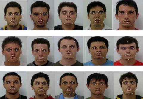
The FEI face database is a Brazilian face database contains a set of face images taken between June 2005 and March 2006 at the Artificial Intelligence Laboratory of FEI in São Bernardo do Campo, São Paulo, Brazil. There are 14 images for each of 200 individuals. In this paper from 2800 images, we only used 60 one. All images are colorful and taken against a white homogenous background in a frontal position with profile rotation of up to about 180 degrees. All faces are mainly represented by students and staff at FEI, ranging between 19 and 40 years old with a distinct appearance, hairstyle. Figure 1 shows some images of the unattractive face database. All images are from a certain angle and young people with age conditions in a certain range.
Figure 1. Example of an image from the unattractive face database
2.1.2 Attractive face database
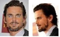
The attractive face database has been collected from the internet, which has labeled as an attractive individual, is confirmed by the film that is named 100 handsome men all over the world on YouTube site. Figure 2 shows some images of the attractive face database. To analyze the images, first, all the images were resized and then if the images were noisy, they were filtered by noise removal techniques [12].
Figure 2. Example of an image from the attractive face database
2.2 Proposed method
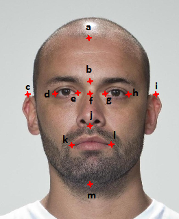
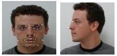
There are different features that can affect facial attraction. For example, the color of the skin, eye colors, face shape, and the geometric features will prepare the facial attractiveness the main point is geometrical features which we focus on base on science. Before defining features, we introduced landmark points of the face. Landmark points can be used as the geometric feature of the face. Landmark is applied extensively in biology, statistical shape analysis, and anthropology. We present an example of a facial image and the geometric landmark coordinates in Figure 3. And it shows 13 landmark points, which name of respectively is:
a) Hairline(forehead); b) Glabella(eyebrow); c, i) Top of the ear s; d, g) Outer canthus; e, h) Inner canthus; f) selion (radix); j) subnasale (nose lip); k, l) Outer commissure; m) menton (chin)
Figure 3. The landmarks on the face used to define its geometric feature
2.2.1 Geometric features
In this section, will see the features extracted from the face in two different poses (frontal and lateral).
These features are extracted based on the calculation of different distances and angles between different landmarks on the face.
(1) Horizontal and vertical lines
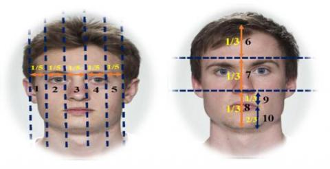
F1) Six vertical lines should cut the face into five equal parts: the distance from the ear to the outer canthus has to be the same size in both sides of the face, and both eyes are equal width, and the width is the same with the distance between eyes. In fact, when we draw a line of correspondence through the face, both sides are concurrent. Figure 4 (at left) shows an example of our considered faces based on features 1 to 5.
F2) Two horizontal lines divide the face into three equal parts: one line goes through the glabella points, the second goes through the subnasale points. The length of the face is divided into three parts, the upper one (trichion) is from forehead to eyebrows, the middle (glabella) is from eyebrows to nose lip, and the lower (menton) is from nose lip to chin. Then, the distance from the top of the forehead to chin. The mentioned distances are equal, and the length of the mouth is 1/3 the distance between the nose and chin. Figure 4 (at right) shows an example of our considered faces based on features 6 to 10.
(2) The distance between facial components
F3) the First distance is between the outer canthus and outer corner points on both sides of the face are equal. The corners width of the mouth aligns with the distance between pupils. Figure 5 (at left) shows the distance described. Based on features 11 to 15.
F4) the distance is the width part of the lip is the same as the distance between the outer canthus. The length of the nose is an equal length of the ears. Figure 5 (at right) shows the distance described based on features 16 to 20.
(3) The angle between facial components
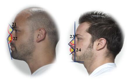
F5) nasofrontal (α) and nasomental (β) angle: For computed of nasofrontal angle, is required to have two lines in the side view of the face, one line goes through the glabella and selion (radix) points and the second line goes through the selion (radix) and pronasale (tip of the nose) points, the angle made is with the name of nasofrontal. For computed nasomental angle, it needs to have two lines in the side view of the face, the first line goes through the selion (radix) and pronasale points, and the second line goes through the pronasale and menton points. These lines together can make of nasomental angle. Figure 6 (at left) shows the angles described based on features 21(α) and 22(β).
F6) nasofacial (γ) and nasolabial (θ) angle: For computed of nasofacial angle, it needs to have 2 lines in the side view of the face, the first line goes through the selion and pronasale points and the second line goes through the pronasale and outer commissure points. These lines together can make of nasofacial angle. Nasolabial angle shows the connection between the nose and the upper lip, using two lines and 3 points Figure 6 (at right) Shows the angles described based on features 23(γ) and 24(θ).
Figure 4. Vertical (at left) and horizontal (at right) dividing of the face image
Figure 5. Some of the geometric features based on indicating the distance between points of the face (landmark)
Figure 6. Some of the geometric features based on indicate four angles between points of the face (landmark)
2.2.2 Artificial Neural Network
Neurons are simple computation units, a collection of several them is known as an artificial neural network, which attempts to model information processing capabilities of the neuron system [13].
To design a machine learning neural network to recognizes faces you may need to undergo a transformation for all the pixels into new ones. The new basis should describe specific face fine details (e.g.: interpupillary distance of landmarks).
Machine learning process for neural networks targets to focus on the set of bases vectors related to the most important faces’ landmarks.
We used error back propagation algorithm as a common method for training a neural network. Network training is stopped when the mean square error (MSE) reaches zero or close to zero or the number of epochs is maximized. We used from a normal distribution [–x, +x] with the mean zero and the standard deviation $\mathrm{x}=\sqrt{\frac{2}{\text { input }+\text { output }}}$. In this paper, we used two methods including the MLP and the SVM to classify attractive people, which we will explain below. Table 1 shows the features extracted from the face. Details of each feature were listed above.
Table 1. A summary of representative features
|
Features type |
pose |
Feature region |
Representative feature |
|
Geometric(F1) |
Frontal |
Whole face |
5 distance(features 1 to 5) between specified landmarks |
|
Geometric (F2) |
Frontal |
Whole face |
5 distance(features 6 to 10) from 7 landmarks |
|
Geometric (F3) |
Frontal |
Ears, eyes, lip |
5 distance (features 11 to 15) from landmarks |
|
Geometric (F4) |
Frontal |
Ears, nose, mouth |
5 distance(features 16 to 20) between landmarks |
|
Geometric (F5) |
Lateral |
Nose, forehead |
2 angle(features 21 and 22) from specified landmarks |
|
Geometric (F6) |
Lateral |
Nose, mouth |
2 angle(features 23 and 24) between landmarks |
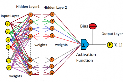
Figure 7. Schematic of the structure of the neural network used in this article to classify attractive and unattractive individuals
(1) Multi-layer perceptron neural network (MLP_NN)
Multi-layer perceptron is one of the classical types of neural networks and is computational techniques used supervised learning. The MLP multi-layer perceptron structure consists of three layers, the input layer, one or more hidden layers, and the output layer. One of the functions of mean squared error is to compare computed and desired values as an approach for learning MLP. In most cases, The MLP neural network is used more for image analysis biometric features, dentistry, various surgeries and etc. This neural network is trained based on user errors and test results. The number of neurons is equaled to the number of features and output layer consists a neuron that produced values between zero and one [14].
Also, in this study we used MLP network for classification. The activation function in all neuros was sigmoid function. The initial weights and initials bias values were set to zero. to train the network Scaled conjugate gradient backpropagation was utilized. Figure 7 shows the structure of the neural network used in this study. The number of neurons in input layer is equal to the number of features extracted from the face. This network is made up of two hidden layers, the first hidden layer of which contains 15 neurons and for the second hidden layer, 10 neurons are considered and in the output layer, one neuron is placed, which shows whether the person is attractive or unattractive [15].
In this network, according to the number of individuals, which is limited to 60 and adapted with the K- Fold method. The network is taught in 3 steps, in each one, there are 20 data which is selected as a test, and the remainder is selected for training. Finally, the errors of each step and the accuracy, specificity, sensitivity of the network are measured, and the average used for making results [16].
2.2.3 Principal component analysis
For saving time and storage, the dimensionality reduction process is useful, to have this purpose with a high level-up accuracy Principal Component Analysis (PCA) can be used.
The PCA has been extensively employed to face feature reduction algorithms and we showed that modular PCA improves the accuracy of face classification. PCA not only reduces the dimensionality of the image but also retains some of the variations in the image data [16].
The data which is used in the analysis should be standardized for having a normal distribution of all variable. So, after using the PCA method, we normalize the obtain properties to equalize the domain of the numbers as the formula. In this paper, PCA used for reducing the dimension of geometric features of the face [16].
In fact, PCA is the statistical method that aims to make data visualization and navigation a simple process. It focuses on extracting smaller number of uncorrelated variables (Principal Components) from a huge number of variables found in huge datasets. The main target is to get the maximum the maximum variance amount with the least number of principal components.
There are algorithms able to reduce the number of features by choosing the most important ones that still represent the entire dataset. One of the advantages pointed out by authors is that these algorithms can improve the results of the classification task.
The PCA is used to describe a large dimensional space with a relatively small set of vectors. PCA is a technique for feature extraction, so the input features combine in a certain method, then we can remove the least important features while still retaining the most valuable parts of all the features. Each of the new features after PCA is independent of each other. This is an advantage because linear model assumptions require that our independent features remain independent of each other. If we decide to fit a linear regression model with these new features, this assumption will necessarily be satisfied.
2.2.4 Evaluation
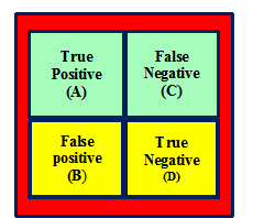
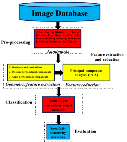
In this system, MLP classifier performance is evaluated on the test set using accuracy, sensitivity, and specificity defined as follows. With true negative (TN), true positive (TP), false positive (FP), and false-negative (FN), corresponding to unattractive, attractive, unattractive, and attractive events, respectively [20]. Figure 8 shows this issue. Eqns. (1, 2, and 3) shows how to calculate sensitivity, specificity, and accuracy. In addition, Figure 9 shows the different steps of the proposed algorithm as a block diagram.
Figure 8. Confusion matrix
Sensitivity $=\frac{A}{A+C}$ (1)
Specificity $=\frac{D}{D+B}$ (2)
Accuracy $=\frac{D+A}{A+B+C+D}$ (3)
Figure 9. The block diagram for Identify Attractive and Unattractive Individuals
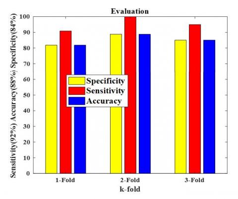
In this section, the evaluation of facial attractiveness was done on 60 faces of men dataset. As it was already mentioned, this data set includes 30 attractive and 30 unattractive face image with 24 geometric features. We first normalized out training data using the mean and Standard Deviation Technique. Then this normalized data were used to improve Multi-Layer Perceptron ANN performances. By using the Normalization technique together with Neural Networks, we developed feature extracted that is able to classify 2 face types (attractive or not) with a very high accuracy rate. One of the best structures for the neural network is shown in Table 2. In this paper, Eighty percent of records (40 images) were used for training, and twenty percent of records (2o image) were used for testing. Experimental results are taken as the average of 30 runs and measured in terms of classification accuracy Training parameters that gave us the highest accuracy can be seen in Table 3, and Figure 10 described this section using a bar plot. The accuracy results vary depending on the participants, with a confidence level of 95% accuracy to the face image rank test. In the 2-class classification, the proposed method achieves improvement in average accuracy ranging from 85% to 95%.
Table 4 shows an example of the results of obtaining 24 geometric features on the attractive and unattractive faces.
Table 2. Structure of a neural network
|
Features |
F1 |
F2 |
F3 |
F4 |
F5 |
F6 |
|
Input |
3 |
5 |
5 |
6 |
4 |
4 |
|
Hidden layer1 |
4 |
5 |
4 |
6 |
6 |
5 |
|
Hidden Layer2 |
3 |
4 |
4 |
3 |
5 |
6 |
|
Training Function |
trainlm |
trainlm |
traincgf |
trainlm |
Traincgf |
traincgf |
|
Learning Function |
learngdm |
learngdm |
learngdm |
learngd |
learngdm |
learngdm |
|
Transfer Function |
tansig |
ansig |
logsig |
tansig |
Tansig |
tansig |
Table 3. Validation classification (attractive or not) in 3 steps and average them
|
k-fold |
Specificity (%) |
Sensitivity (%) |
Accuracy (%) |
|
1 |
81.81 |
88.88 |
85 |
|
2 |
90.90 |
100 |
95 |
|
3 |
81.81 |
88.88 |
85 |
|
total |
84 |
92 |
88 |
Table 4. An example of all the geometric features used in the paper
|
Features |
Attractive men |
Unattractive men |
|
1 |
2.7335 |
2.1389 |
|
2 |
3.4931 |
3.5507 |
|
3 |
3.4948 |
4.2621 |
|
4 |
3.4977 |
3.3664 |
|
5 |
3.1750 |
2.1984 |
|
F1 (mean1-5) |
3.2788 |
3.1033 |
|
6 |
7.3704 |
6.7788 |
|
7 |
6.0963 |
6.7853 |
|
8 |
9.2712 |
7.4275 |
|
9 |
2.5408 |
2.4528 |
|
10 |
6.6675 |
5.1010 |
|
F2 (mean6-10) |
6.8590 |
5.9844 |
|
11 |
5.2705 |
5.1675 |
|
12 |
5.3990 |
5.6817 |
|
13 |
10.5410 |
11.0446 |
|
14 |
7.0488 |
7.6178 |
|
15 |
5.8420 |
5.1675 |
|
F3 (mean11-15) |
6.8202 |
6.9358 |
|
16 |
5.7277 |
5.0451 |
|
17 |
6.9890 |
7.8402 |
|
18 |
4.3185 |
5.4900 |
|
19 |
6.9343 |
7.9813 |
|
20 |
5.9069 |
5.1739 |
|
F4 (mean16-20) |
5.97528 |
6.3061 |
|
21 |
112.0733 |
127.2348 |
|
22 |
137.4451 |
138.0536 |
|
F5 (mean 21,22) |
124.7592 |
132.6442 |
|
23 |
93.6309 |
99.4823 |
|
24 |
72.4016 |
95.9888 |
|
F6(mean 23,24) |
83.01625 |
97.7355 |
Figure 10. Sensitivity, specificity, and accuracy evaluated by MLP classifier
The purpose of this article is to classify individuals and identify whether a person is attractive or not. The results showed that geometric features are important for facial attractiveness diagnosis, and the different values of this feature can affect the amount of facial attractiveness.
Although determining each person's value based on beauty and physical attraction causes distress and injustice, but never this kind of approach to individuals destroy. Thus, it is necessary to introduce a feature which is playing a role in facial attractiveness.
Not only the geometric features and scientific index for the detection of attractive and unattractive individuals are examined, but also we use neural network classification for making much more distinction.
Facial attractiveness analysis emerges from researches with the topic of pattern recognition, image processing, and computer vision.
Furthermore, geometric features based on facial beauty analysis attracted the attention of researchers from psychology, the biometric community, and computer science. In addition, it also has some benefits for society, which has many potential applications such as aesthetic plastic surgery planning, cosmetic advertising, photo editing, and entertainment.
[1] Zhang, L., Zhang, D., Sun, M.M., Chen, F.M. (2017). Facial beauty analysis based on geometric feature: Toward attractiveness assessment application. Expert Systems with Applications, 82: 252-265. https://doi.org/10.1016/j.eswa.2017.04.021
[2] Shi, J., Samal, A., Marx, D. (2006). How effective are landmarks and their geometry for face recognition? Computer Vision and Image Understanding, 102(2): 117-133. https://doi.org/10.1016/j.cviu.2005.10.002
[3] Chen, F., Zhang, D. (2016). Combining a causal effect criterion for evaluation of facial attractiveness models. Neurocomputing, 177: 98-109. https://doi.org/10.1016/j.neucom.2015.11.010
[4] Jones, B.C., DeBruine, L.M., Little, A.C. (2007). The role of symmetry in attraction to average faces. Perception & Psychophysics, 69(8): 1273-1277. https://doi.org/10.3758/BF03192944
[5] Schmid, K., Marx, D., Samal, A. (2008). Computation of a face attractiveness index based on neoclassical canons, symmetry, and golden ratios. Pattern Recognition, 41(8): 2710-2717. https://doi.org/10.1016/j.patcog.2007.11.022
[6] Kagian, A., Dror, G., Leyvand, T., Meilijson, I., Cohen-Or, D., Ruppin, E. (2008). A machine learning predictor of facial attractiveness revealing human-like psychophysical biases. Vision Research, 48(2): 235-243. https://doi.org/10.1016/j.visres.2007.11.007
[7] Zhang, D., Zhao, Q., Chen, F. (2011). Quantitative analysis of human facial beauty using geometric features. Pattern Recognition, 44(4): 940-950. https://doi.org/10.1016/j.patcog.2010.10.013
[8] Nguyen, T.V., Liu, S., Ni, B., Tan, J., Rui, Y., Yan, S. (2013). Towards decrypting attractiveness via multi-modality cues. ACM Transactions on Multimedia Computing, Communications, and Applications (TOMM), 9(4): 1-20. https://doi.org/10.1145/2501643.2501650
[9] Fan, J., Chau, K. P., Wan, X., Zhai, L., Lau, E. (2012). Prediction of facial attractiveness from facial proportions. Pattern Recognition, 45(6): 2326-2334. https://doi.org/10.1016/j.patcog.2011.11.024
[10] Phillips, P.J., Wechsler, H., Huang, J., Rauss, P.J. (1998). The FERET database and evaluation procedure for face-recognition algorithms. Image and Vision Computing, 16(5): 295-306. https://doi.org/10.1016/S0262-8856(97)00070-X
[11] https://www.boredpanda.com/top-100-most-handsome-men-faces-2018-tc-candler/, accessed on August 21 2019.
[12] Mateen, M., Wen, J., Song, S., Huang, Z. (2019). Fundus image classification using VGG-19 architecture with PCA and SVD. Symmetry, 11(1): 1. https://doi.org/10.3390/sym11010001
[13] Alickovic, E., Subasi, A. (2019). Normalized neural networks for breast cancer classification. In International Conference on Medical and Biological Engineering, pp. 519-524. https://doi.org/10.1007/978-3-030-17971-7_77
[14] Sharifzadeh, F., Akbarizadeh, G., Kavian, Y.S. (2019). Ship classification in SAR images using a new hybrid CNN–MLP classifier. Journal of the Indian Society of Remote Sensing, 47(4): 551-562. https://doi.org/10.1007/s12524-018-0891-y.
[15] Souza, J.F.L., Santos, M.D., Magalhães, R.M., Neto, E. M., Oliveira, G.P., Roque, W.L. (2019). Automatic classification of hydrocarbon “leads” in seismic images through artificial and convolutional neural networks. Computers & Geosciences, 132: 23-32. https://doi.org/10.1016/j.cageo.2019.07.002
[16] Hanbay, D., Turkoglu, I., Demir, Y. (2008). An expert system based on wavelet decomposition and neural network for modeling Chua’s circuit. Expert Systems with Applications, 34(4): 2278-2283. https://doi.org/10.1016/j.eswa.2007.03.002