Vimala Kumari Gollu* | Ganta Usha Sravani | Mandru Sunil Prakash | Ganta Srikanth
© 2021 IIETA. This article is published by IIETA and is licensed under the CC BY 4.0 license (http://creativecommons.org/licenses/by/4.0/).
OPEN ACCESS
In recent times, medical scan images are crucial for accurate diagnosis by medical professionals. Due to the increasing size of the medical images, transfer and storage of images require huge bandwidth and storage space, and hence needs compression. In this paper, multilevel thresholding using 2-D histogram is proposed for compressing the images. In the proposed work, hybridization of optimization techniques viz., Genetic Algorithm (GA), Particle Swarm Optimization (PSO) and Symbiotic Organisms Search (SOS) is used to optimize the multilevel thresholding process by assuming the Renyi entropy as an objective function. Meaningful clusters are possible with optimal threshold values, which lead to better image compression. For performance evaluation, the proposed work has been examined on six Magnetic Resonance (MR) images of brain and compared with individual optimization techniques as well as with 1-D histogram. Recent study reveals that peak signal to noise ratio (PSNR) fail in measuring the visual quality of reconstructed image because of mismatch with the objective mean opinion scores (MOS). So, we incorporate weighted PSNR (WPSNR) and visual PSNR (VPSNR) as performance measuring parameters of the proposed method. Experimental results reveal that hGAPSO-SOS method can be accurately and efficiently used in problem of multilevel thresholding for image compression.
genetic algorithm (GA), image compression, image thresholding, particle swarm optimization (PSO), symbiotic organisms search (SOS), 2-D histogram
Medical images are an efficient source for better diagnosis of the disease and also help in assessing the severity of the disease. Their effective transmission of the diagnosis details through telemedicine benefits rural areas at times of emergencies or doctors’ absence or unavailability of the infrastructure. They play a significant part in identifying internal structure of the human body and helps understand the affected areas. But due to their increasing size, transfer and storage requires huge bandwidth and storage space, hence needs compression. Image compression reduces size of the image or video that is to be transmitted by removing irrelevant or repeated bits, so that image can be stored and transmitted in an efficient form and it reduces the Bits per Pixel (BPP), and maintain quality in reconstructed image. In general, images of the medical scan can be compressed in two ways: lossless compression and lossy compression. As the images that are to be provided for physicians and surgeons need to be of high quality and as lossless compression techniques provide low compression ratio it is quite difficult to transmit large amounts of data. In such a condition, lossy compression technique that comes with good compression ratio is needed. Therefore, it is essential to derive effective compression algorithms which have minimal loss, less time complexity, increased reduction in size and still preserve a significant amount of quality in reconstructed image. To achieve this, Various strategies for Image compression are developed and is ordered into two classes, with and without transform technique. JPEG is the principal global lossy transformed approach and is advantageous for consistent tone still gray scale and color image compression. International Organization for Standardization (ISO) and International Electro-specialized Commission (IEC) together presented JPEG in 1992 [1]. DCT is utilized as transform technique in JPEG image compression. The element of DCT is that the large portion of the energy is focused on D.C coefficients and in low frequency sub-band [2]. After progressive creation of DWT, image compression has been moved to next stage which offers enhanced reformed image quality with high compression [3, 4]. Due to tedious coding measure, the computational complexity of JPEG-2000 is slower than JPEG by 30 times [5, 6].
Quantization is of two types: scalar quantization and vector quantization. When compared to scalar quantization, execution of Vector Quantization (VQ) procedure is superior. VQ is essentially a C-means clustering technique broadly utilized for image compression [7]. Linde et al. presented the Linde–Buzo–Gray (LBG) algorithm, which starts with the lowest codebook size and bit by bit increment size of codebook, utilizing a parting system [8] to progress the enactment of c-means. LBG algorithm is simple, adaptable and flexible but, does not guarantee the best global solutions. Recently, the evolutionary optimization algorithms had been developed to design the codebook for improving the results of LGB algorithm. Rajpoot et al. designed a codebook by using an ant colony system (ACS) algorithm [9]. Moreover, vector quantization using particle swarm optimization (PSO) [10] beats LBG algorithm, which depends on solution of updating the global best (gbest) and local best (lbest). Wang et al. developed Quantum particle swarm algorithm (QPSO), to tackle the 0–1 backpack issue [11]. Kumari et al. proposed Flower Pollination Algorithm (FPA) for efficient codebook design to compress the medical images [12]. Vector quantization is one which is utilized for clustering the image and data. But due to time consuming procedure, design of codebook is troublesome task [13]. Fractal image compression is a non-transformation technique where image is changed into more modest locales for improved image compression however this procedure is totally tedious [14]. Another non-transformation technique is Artificial Neural Networks, is accomplished for image compression by the neural organization; the outcomes are demonstrated that the training algorithm and the back propagation neural organization can expand the performance [15, 16]. Mardani et al. have used Generative Adversarial Neural Networks (GANs) based compressive sensing framework to model the (low-dimensional) manifold of high-quality MR images [17]. Gözcü et al. have proposed a learning-based framework for optimizing MRI subsampling patterns for a specific reconstruction rule and anatomy [18]. Gao and Xiong have proposed a deep learning framework for the enhancement of compressed brain images [19]. Another non-transformation procedure is thresholding. Thresholding is performed as in otsu technique by class variance or depending on the criterion of entropies like Shannon, Fuzzy, and Kapur [20, 21]. One of inherent thresholding procedure is Birge–Massart, which is utilized for image compression [22]. A weighted membership function is altered by the spatial information of local and global to improve the results of thresholding MR images in conditional spatial FCM [23]. CT images are segmented by SVM using various kernel functions and optimization of sequential minimal using threshold optimization [24-26].
Kumari et al. proposed Hybrid Bacteria Foraging Optimization Algorithm and Particle Swarm Optimization (HBFOA–PSO) algorithm for effective outcomes of thresholding to achieve improved image compression [27]. Ahilan et al. have proposed the use of PSO and its variants Darwinian PSO and Fractional Order DPSO algorithms for multi-level thresholding for image segmentation for lossless compression of medical images [28]. Hoang et al. proposed a new layered image compression framework with encoder-decoder matched semantic segmentation (EDMS) and shows better results when compared to the state-of-the-art semantic-based image codec [29]. A serious problem of first-order thresholding using 1-D histogram is that the spatial correlation between pixels is not considered. Recent investigations show that the outcomes acquired with 2D histogram oriented methodologies are better than those got with 1D histogram [30]. Farnad et al. have shown that hybrid PSO/GA/SOS algorithm (HPG-SOS) dominates other evolutionary algorithms in terms of convergence, execution time and success rate [31]. This work, therefore, proposes the use of Hybrid Genetic Algorithm Particle Swarm Optimization Symbiotic Organisms Search (hGAPSO-SOS) for effective and efficient 2-D histogram based multilevel thresholding for the first time, for image compression. Multilevel thresholding is developed using 2-D histogram by assuming the Renyi entropy as an objective function. Meaningful/useful clusters are possible with optimal threshold values, which lead to better image thresholding and thereby to the objective of image compression. The obtained results are compared with individual optimization techniques such as Grey Wolf Optimization (GWO), Moth-flame Optimization (MFO), Flower Pollination Optimization (FPO), Particle Swarm Optimization (PSO), Bacteria Foraging Optimization Algorithm (BFOA), and Hybrid Bacteria Foraging Optimization Particle Swarm Optimization (HBFOA-PSO) and, with 1-D histogram. For the performance evaluation of the proposed work, Peak Signal to Noise Ratio (PSNR), Weighted Peak Signal to Noise Ratio (WPSNR), objective function, Visual PSNR (VPSNR), and Compression Ratio (CR) are considered. In every parameter, the performance of proposed hGAPSO-SOS algorithm with 2-D histogram is better than other state of the art algorithms and, with 1-D histogram.
This paper is organized as follows: Section 2 describes the objective function Renyi Entropy. In Section 3, the algorithms GA, PSO and SOS are explained. The proposed approach is explained in Section 4. Finally, results are discussed in Section 5 followed by Conclusion in Section 6.
For additive and independent random events, consider ‘n’ array discrete probability distributions (pdf) as (F1, F2, F3 … Fn) ε Δn where Δn={(F1, F2, F3 … Fn), Fi≥0, and $\sum_{i=1}^{n} F_{i}=1$} for random variables (X1, X2, X3, …… Xn) then Renyi entropy is given as
$\mathop{H}_{\alpha }=\frac{1}{1-\alpha }\mathop{\log }_{2}\left( \sum\nolimits_{i}^{n}{\mathop{F}_{i}^{\alpha }} \right)$ (1)
Here ‘α’ is higher than zero and, is approaches towards to one, the Renyi entropy turn out to be Shannon entropy. Basically, image is clustered into two, one conveys object data (cluster C1) and another conveys background (cluster C2), at that point Renyi entropy is
$\mathop{H}_{\alpha }\left[ \mathop{C}_{1} \right]=\frac{1}{1-\alpha }\left[ \mathop{\log }_{2}\left( \sum\nolimits_{i=0}^{t}{\mathop{\left( \frac{F\left( i \right)}{F\left( \mathop{C}_{1} \right)} \right)}^{\alpha }} \right) \right]$ (2)
$\mathop{H}_{\alpha }\left[ \mathop{C}_{2} \right]=\frac{1}{1-\alpha }\left[ \mathop{\log }_{2}\left( \sum\nolimits_{i=t+1}^{L-1}{\mathop{\left( \frac{F\left( i \right)}{F\left( \mathop{C}_{2} \right)} \right)}^{\alpha }} \right) \right]$ (3)
where, $F\left(C_{1}\right)=\sum_{i=0}^{t} F(i), F\left(C_{2}\right)=\sum_{i=t+1}^{L-1} F(i)$, Here Fi is the normalized histogram of image and, ‘L’ is highest intensity level of gray scale image. With single threshold value ‘t’, the Renyi entropy is given as
$\mathop{\phi }_{\alpha }\left( t \right)={{\arg }_{\max }}\left( \left[ \mathop{H}_{\alpha }\left[ \mathop{C}_{1} \right]+\mathop{H}_{\alpha }\left[ \mathop{C}_{2} \right] \right] \right)$ (4)
2.1 Concept of multi-level thresholding
With ‘N’ threshold values, t=(t1, t2, t3 … tN), the image be portioned into ‘N’ clusters C=(C1, C2, C3 … CN). The Renyi entropy for every distinct cluster is characterized as
$\mathop{H}_{\alpha }\left[ \mathop{C}_{1} \right]=\frac{1}{1-\alpha }\left[ \mathop{\log }_{2}\left( \sum\nolimits_{i=0}^{\mathop{t}_{1}}{\mathop{\left( \frac{F\left( i \right)}{F\left( \mathop{C}_{1} \right)} \right)}^{\alpha }} \right) \right]$ (5)
$\mathop{H}_{\alpha }\left[ \mathop{C}_{2} \right]=\frac{1}{1-\alpha }\left[ \mathop{\log }_{2}\left( \sum\nolimits_{i=\mathop{t}_{1}+1}^{\mathop{t}_{2}}{\mathop{\left( \frac{F\left( i \right)}{F\left( \mathop{C}_{2} \right)} \right)}^{\alpha }} \right) \right]$ (6)
$\mathop{H}_{\alpha }\left[ \mathop{C}_{N} \right]=\frac{1}{1-\alpha }\left[ \mathop{\log }_{2}\left( \sum\nolimits_{i=\mathop{t}_{N}-1}^{L-1}{\mathop{\left( \frac{F\left( i \right)}{F\left( \mathop{C}_{N} \right)} \right)}^{\alpha }} \right) \right]$ (7)
where, $F\left(C_{1}\right)=\sum_{i=0}^{t_{1}} F(i), \quad F\left(C_{2}\right)=\sum_{i=t_{1}+1}^{t_{2}} F(i)$ and $F\left(C_{N}\right)=\sum_{i=t_{N}^{-1}}^{L-1} F(i)$.
With ‘N’ thresholds, the overall Renyi entropy or objective function of image is given as
$\mathop{\phi }_{\alpha }\left( t \right)={{\arg }_{\max }}\left( \left[ \begin{align} & \mathop{H}_{\alpha }\left[ \mathop{C}_{1} \right]+\mathop{H}_{\alpha }\left[ \mathop{C}_{2} \right] +\cdots \mathop{H}_{\alpha }\left[ \mathop{C}_{N} \right] \\\end{align} \right] \right) $ (8)
Two fake thresholds are presented t0 and tN=L-1 which have the condition t0 < t1………. < tN-1 < tN to make simpler calculations. The optimal thresholds are attained with any soft computing technique by maximizing the Eq. (8).
2.2 Two-dimensional Renyi entropy
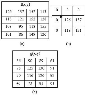
Consider I(m, n) is an intensity of image at spatial location (m, n) with size of the image as ‘M×N’ for gray scale image, and its 1D-histogram is ‘h(x)' for x ε {1, 2, 3,……., L-1}, here ‘L’ is 256 with elements in histogram as G. In literature, 1D-histogram is used for selection of optimal thresholds and are attained by optimizing the objective function i.e. entropy. The 2-D histogram of an image is found by characterizing a local average of nine neighboring pixels, I(x, y), denoted g(x, y) as
$g\left( x,y \right)=\frac{1}{9}\sum\nolimits_{i=-1}^{1}{\sum\nolimits_{j=-1}^{1}{f\left( x+i,y+j \right)}}$ (9)
Figure 1. Sample for 2-D histogram calculation
For instance let us take an image of size 4×4 as appeared in Figure 1(a) and its average intensity g(x, y) is determined by padding required number of zeros at edges as appeared in Figure 1(b) for first element i.e. 126 of Figure 1(a), and is given in Figure 1(c).
The 2-D histogram computed using Eq. (9) of the marked area of Metastatic image is shown in Figure 2. It is divided/grouped into four clusters by a single threshold (t, s), where ‘t’ and ‘s’ are thresholds for original image I(x, y) and average image g(x, y) respectively. The area of divided clusters is not the same. From the 2-D histogram, it is seen that corner to corner quadrants convey a lot of data. The diagonal 1st quadrant indicates object, 3rd background and 2nd, 4th quadrants are ignored because they do not convey any information.
Figure 2. Metastatic image and 2-D histogram
For object and background quadrants, Renyi entropy is given as
$\begin{align} & \mathop{H}_{object}^{\alpha }\left[ t,s \right]=\frac{1}{1-\alpha }\left[ \mathop{\log }_{2}\sum\nolimits_{i=0}^{t}{\left( \sum\nolimits_{j=0}^{s}{\mathop{\left( \frac{F\left( i,j \right)}{\mathop{F}_{D1}\left( t,s \right)} \right)}^{\alpha }} \right)} \right] \\\end{align}$ (10)
$\begin{align} & \mathop{H}_{background}^{\alpha }\left[ t,s \right]=\frac{1}{1-\alpha }\left[ \mathop{\log }_{2}\sum\nolimits_{i=t+1}^{L-1}{\left( \sum\nolimits_{j=s+1}^{L-1}{\mathop{\left( \frac{F\left( i,j \right)}{\mathop{F}_{D2}\left( t,s \right)} \right)}^{\alpha }} \right)} \right] \\\end{align}$ (11)
where, $F_{D 1}(t, s)=1-\sum_{i=0}^{t} \sum_{j=0}^{s} F(i, j)$ and, $F_{D 2}(t, s)=$ $1-\sum_{i=t+1}^{L-1} \sum_{j=s+1}^{L-1} F(i, j)$.
For optimum threshold (t, s) selection, the objective function which is to be maximized is
$\mathop{\phi }_{\alpha }\left( t \right)={{\arg }_{\max }}\left( \left[ \mathop{H}_{object}^{\alpha }\left[ t,s \right]+\mathop{H}_{background}^{\alpha }\left[ t,s \right] \right] \right)$ (12)
2.3 Multi-level thresholding using 2D-hisotgram
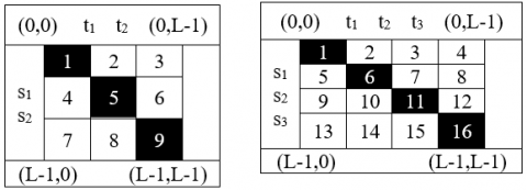
Thresholding with 2-D histogram conveys superior outcomes particularly in multilevel thresholding. Multilevel thresholding picked up lots of popularity over bi-level thresholding because; it clusters the image into several suitable clusters, helps in precise examination and interpretation of the image [36]. With two thresholds (t1, t2) and (s1, s2), the 2-D histogram of an image is clustered into 9 clusters as appeared in Figure 3(a). At that point the slanting quadrants first, fifth and ninth represents objects(s) regions, intermediate and background respectively as shown in Figure 3(a) and other regions are noise and edges and are neglected. The 2-D histogram of an image is clustered into 16 clusters with three thresholds (t1, t2, t3) and (s1, s2, s3) as shown in Figure 3 (b).
Figure 3. 2-D histogram: a) 2- level b) 3- level
With two thresholds, Renyi entropy of diagonal quadrants are calculated as
$\begin{align} & \mathop{H}_{object}^{\alpha }\left[ t,s \right]=\frac{1}{1-\alpha }\left[ \mathop{\log }_{2}\sum\nolimits_{i=0}^{\mathop{t}_{1}}{\left( \sum\nolimits_{j=0}^{\mathop{s}_{1}}{\mathop{\left( \frac{F\left( i,j \right)}{\mathop{F}_{D1}\left( t,s \right)} \right)}^{\alpha }} \right)} \right] \\\end{align}$ (13)
$\begin{align} & \mathop{H}_{\operatorname{int}ermediate}^{\alpha }\left[ t,s \right]=\frac{1}{1-\alpha }\left[ \mathop{\log }_{2}\sum\nolimits_{\mathop{t}_{1}+1}^{\mathop{t}_{2}}{\left( \sum\nolimits_{\mathop{s}_{1}+1}^{\mathop{s}_{2}}{\mathop{\left( \frac{F\left( i,j \right)}{\mathop{F}_{D2}\left( t,s \right)} \right)}^{\alpha }} \right)} \right] \\\end{align}$ (14)
$\begin{align} & \mathop{H}_{background}^{\alpha }\left[ t,s \right]=\frac{1}{1-\alpha }\left[ \mathop{\log }_{2}\sum\nolimits_{\mathop{t}_{2}+1}^{L-1}{\left( \sum\nolimits_{\mathop{s}_{2}+1}^{L-1}{\mathop{\left( \frac{F\left( i,j \right)}{\mathop{F}_{D3}\left( t,s \right)} \right)}^{\alpha }} \right)} \right] \\\end{align}$ (15)
where,
$\begin{array}{ll}F_{D 1}(t, s)=1-\sum_{i=0}^{t_{1}} \sum_{j=0}^{s_{1}} F(i, j),\ F_{D 2}(t, s)=1- \sum_{i=t_{1}+1}^{t_{2}} \sum_{j=s_{1}^{+1}}^{S_{2}} F(i, j) \ \text { and } \ F_{D 3}(t, s)=1- \sum_{i=t_{2}+1}^{L-1} \sum_{j=s_{2}^{+1}}^{L-1} F(i, j), \text { for optimum threshold }(\mathrm{t}, \mathrm{s}) \text { selection, }\end{array}$ the objective function which is to maximize is
$\begin{align} & \mathop{\phi }_{\alpha }\left( t \right)={{\arg }_{\max }} \left( \left[ \mathop{H}_{object}^{\alpha }\left[ t,s \right]+\mathop{H}_{\operatorname{int}ermediate}^{\alpha }\left[ t,s \right]\mathop{+H}_{background}^{\alpha }\left[ t,s \right] \right] \right) \\\end{align}$ (16)
For ‘N’ thresholds, the equation is given as
$\begin{align} & \mathop{\phi }_{\alpha }\left( t \right)=\arg \max \left( \left[ \mathop{H}_{1}^{\alpha }\left[ t,s \right]+\mathop{H}_{2}^{\alpha }\left[ t,s \right]\mathop{+H}_{3}^{\alpha }\left[ t,s \right]\cdots \mathop{+H}_{N+1}^{\alpha }\left[ t,s \right] \right] \right) \\\end{align}$ (17)
where,
$\begin{align} & \mathop{H}_{K}^{\alpha }\left[ t,s \right]=\frac{1}{1-\alpha } \left[ \mathop{\log }_{2}\sum\nolimits_{\mathop{i=t}_{K-1}+1}^{\mathop{t}_{K}}{\left( \sum\nolimits_{\mathop{s}_{K-1}+1}^{\mathop{s}_{K}}{\mathop{\left( \frac{F\left( i,j \right)}{\mathop{F}_{DK}\left( t,s \right)} \right)}^{\alpha }} \right)} \right] \\\end{align}$ (18)
Two dummy variables are selected t0 and tN+1= L-1 which fulfill the condition t0 < t1………. < tN-1 < tN+1 for simplifying the calculations. Likewise, s0 and sN+1=L-1 are selected with condition s0 < s1………. < sN-1 < sN+1. The 2-D histogram of four brain MR images is appeared in Figure 4. From the figure, it is seen that the greater part of the data/energy is focused on corner to corner quadrants. Multilevel thresholding is a tedious procedure and is relative to the number of thresholds ‘N’. So, soft computing techniques play a significant role in this challenge by assuming Eq. (17) as an objective function which prompts decrease in the computational time.
Figure 4. Input images and corresponding 2-D histogram
3.1 Genetic Algorithm (GA)
It was initiated and developed between the years 1960s to 1970s by a team called Holland team and is being used for many constrained and unconstrained optimization problems. It is inspired and developed by in-depth study of natural selection of Charles Darwin’s theory [25]. GA being a non-swarm-based technique consists of chromosome for each and every population or solution of the problem. Initial populations are generated by a random number within the range of search space. The ordinary GA uses two steps for selection and creation of new population i.e., mutation operation and crossover operation. The newly generated population or chromosomes are named as offspring. The crossover operation is performed between two parents for generation of new healthy child. Offspring C is calculated from parents A and B, with the following equation,
$\mathop{C}_{i}={{\alpha }_{i}}\mathop{A}_{i}+\left( 1-\alpha \right)\mathop{B}_{i},$ (19)
where, $\alpha_{i} \in[0,1]$ is a random number.
In all iterations, chromosomes change their values by mutation operation. Mutation in real number is obtained by addition of chromosome with randomly created real number or randomly generated number from Gaussian (normal) distribution. Let A is chromosome and it’s ith variable is Ai then new offspring Al is obtained by mutating ith gene Ail and is calculated with the following equation:
$\mathop{A}_{i}^{1}=\mathop{A}_{i}+N,$ (20)
where, ‘N’ is random number or value taken form Gaussian distribution as
$N=rand\left( 0,1 \right)\left[ UB-LB/M \right],$
$L B<A_{i}$ and $A_{i}^{1}<U B$
Here, ‘M’ is random real number (range between 1 and 1000, mostly authors prefer M value 10) and rand (0,1) is a random number lies between 0 to 1. LB and UB are lower limit and upper limit of Ai and Ail respectively.
The genetic algorithm can be explained in the following steps:
Step 1: Initialize number of chromosomes as N.
Step 2: Calculate the objective function/fitness function for all N chromosome.
Step 3: N chromosome are updated by four repeated steps i.e., best chromosome selection – Crossover operation and Mutation operation and finally Replacement.
Step 4: The generated chromosomes are forwarded for next iterations.
Step 5: Repeat step 2 - 4 till stopping criteria or maximum Iteration.
3.2 Particle swarm optimization
It is inspired by the searching behavior of particles; some examples are swarm of fish or birds and was developed in the year 1995 by Eberhart and Kennedy 1995 [25]. The PSO, follows randomness and some intelligence in updation of the both particle positions and velocity. The PSO being a swarm-based optimization and is simple and easily adopted for any particle and mathematical problems. Each particle in PSO may be assumed as one bird or one fish and are indicated with Oi. Each particle gains some initial velocity Vi and position Oi of dimensions equal to dimensions of the problem. In all iterations each particle holds some position called personal best (Op) and highest fitness particle holds global best (Obest) position and these positions are updated in upcoming iterations. Let ‘t’ is current iteration, then PSO velocity and position update follows Eq. (21) and Eq. (22).
$\begin{align} & \mathop{V}_{i,d}\left( t+1 \right)=\mathop{V}_{i,d}\left( t \right)+\mathop{c}_{1}\mathop{r}_{1}\left( \mathop{O}_{p\left( i,d \right)}\left( t \right)-\mathop{O}_{i,d}\left( t \right) \right)+\mathop{c}_{2}\mathop{r}_{2}\left( \mathop{O}_{best\left( d \right)}\left( t \right)-\mathop{O}_{i,d}\left( t \right) \right) \\\end{align}$ (21)
$\mathop{O}_{i,d}\left( t+1 \right)=\mathop{O}_{i,d}\left( t \right)+\mathop{V}_{i,d}\left( t+1 \right)$ (22)
Eq. (21) is for velocity updation and Eq. (22) is for updation of particle position with the help of updated velocities. Op(i, d) is a personal best for particle i and Obest is the best particle among all particle in current iteration ‘t’, c1 and c2 are user defined control tuning parameters, r1 and r2 are random numbers lying between 0 to 1. The PSO algorithm is as follows.
PSO algorithm:
1: Initialize positions of all particles Oi and corresponding velocities Vi.
2: Assign highest fitness particle as Obest
3: While (termination criterion)
4: for i=1, 2,...,n do
5: Update velocities of all particles by using Eq. (21)
6: Update positions of all particles by using Eq. (22)
7: Find new objective function of updated particle Oi(t + 1)
8: If new objective function value Oi(t + 1) is higher than old Op,i(t) then
9: Replace Op,i(t) with Oi(t + 1)
10: end if
11: end for
12: Now find Obest(t) in all updated particles Op(t)
13: itr=itr + 1 (iteration increment)
14: end while
15: Finally, outcome Obest is generated.
3.3 Symbiotic organisms search (SOS)
SOS is a soft computing technique developed based on organisms and was proposed in the year 2014 by Prayogo and Cheng, it is inspired by the natural behavior of symbiotic organisms that used to survive in the ecosystem [28]. The fitness for each organism shows the level of adaption to the treated objective. The major advantage of SOS is, it does not require prior tuning of tuning parameters. As like other algorithms, SOS updates the all organism position in each iteration. Position update is done in three successive operations; those are Mutualism, Commensalism and Parasitism. The organism positions will be changed based on best possible relation among all. The algorithm is summarized as following:
1. Initialize the required parameters
2. While (until stopping criterion) do
Three phases I. Mutualism II. Commensalism III. Parasitism
3. End while
In each iteration, update the phases with the corresponding equations and are as follows.
3.3.1 Mutualism phase
It is a phase, in which both the organisms are benefited, associated with the connection among flowers and honey bees. In this stage, organism Oj randomly selected and it interacts with the other organism Oi. They maintain a good relationship between them so that both organisms get benefited. The updated position of both the organisms is obtained with the following equations.
$\begin{align} & \mathop{O}_{inew}=\mathop{O}_{i}+ rand(0,1)*\left( \mathop{O}_{best}-\left( Mutual\_vector*\mathop{BF}_{1} \right) \right) \\\end{align}$ (23)
$\begin{align} & \mathop{O}_{jnew}=\mathop{O}_{j}+ rand(0,1)*\left( \mathop{O}_{best}-\left( Mutual\_vector*\mathop{BF}_{2} \right) \right) \\\end{align}$ (24)
$Mutual\_vector=\frac{\mathop{O}_{i}+\mathop{O}_{j}}{2}$ (25)
where, mutal_vector gives relationship between the organisms Oi and Oj and above equation explains the efforts of mutualistic in gaining their goals and enhance their living survival. The benefit factors BF1 and BF2 show how much of benefit organism acquired while interacting with another organism. These two are randomly selected and must be either 1 or 2. Obest is the best level of adaption that has established up to this point.
3.3.2 Commensalism phase
This phase is developed on the basis of relation between the Remora fish and sharks. The remora always receives benefits whereas shark may or may not receive benefits from relationship. As discussed in mutualism phase, in this Oi organism gets benefit by maintaining a relationship with randomly selected Oj organism. Then updated equation is (26)
$\mathop{O}_{inew}=\mathop{O}_{i}+rand(-1,1)*\left( \mathop{O}_{best}-\mathop{O}_{j} \right)$ (26)
3.3.3 Parasitism phase
This phase exit between the human being and malaria mosquito, in which human being gets effected and some time may die and mosquitoes get benefited with the relationship. As one of the organisms got effected so there is a need to replace with newly generated organism. As like other phases, one organism is selected arbitrarily Oj and it acts as a victim for parasite vector. In problem search space this vector is obtained by duplicating Oi with newly generated and then modifies the randomly chosen organism. If at all this vector is better as compared to Oj then this phase kills Oj and replace or else Oj gains some energy from parasite and live for some other days.
Three of the evolutionary algorithms GA, PSO and SOS are combined, represented as hGAPSO-SOS, inspired by Charles Darwin’s natural selection for the first time [29]. Here is fact that if any organism has good genetic structure, it leads to a better feature, and has long life in ecosystem. The GA creates a better offspring with good genetic structure from parents. The PSO algorithm gives some important experiences to all organisms which leads better survival of each organism. In the proposed algorithm, PSO follows GA and then SOS follows the sequence.
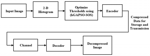
In all iterations, the hGAPSO-SOS starts with GA with required population, dimension of problem and required initialization of parameters. In next step, all organisms get some best experience with PSO. If any organism position is better as compared to past position, then it will move to better level or else it will remain in same position. If best experience is better than the global best Obest, then replace it with new position. So PSO always trying to check for better position by updating the velocity and keep best for the next iterations and also it updates the Obest. As all the organisms got some experience with the PSO, now they try to establish a better relation with other organism which leads to better offspring and healthy population. In third phase, if any organism gets improved fitness value, then that organism position is updated with SOS interaction. From the whole observation the GA and SOS are useful for position update and PSO update the Obest and personal best of organism. If the current iteration is equal to stopping condition then algorithm stop or else same process is repeated. Block diagram of proposed HGAPSO-SOS algorithm for image compression using multilevel thresholding with 2-D histogram is shown in below Figure 5.
Figure 5. Block diagram of image compression using hGAPSO-SOS Algorithm with 2-D histogram
In this paper, Hybridization of GA, PSO, and SOS (HGAPSO-SOS) is used for 2-D histogram by maximizing the Renyi’s entropy for effective and efficient image thresholding for image compression. For evaluation of the experiments the method adopted for design of thresholds with the assistance of both 1-D and 2-D histogram is gray scale image coding. Six Magnetic Resonance Imaging (MRI) brain images of four diverse patients with age 3, 32, 35, and 42 taken from BraTS dataset 2018 of size 256 × 256 namely “Astrocytoma”, “Coronary T1 Astrocytoma”, “Glioma”, “Metastatic”, “PNET”, and “Meningioma’’ are adopted for valuation of compression and each pixels take 8 bits (bits per pixel=8). The programs are implemented using Matlab15a with 100 initial solutions. The performance of the proposed hGAPSO-SOS algorithm is compared with six different algorithms namely GWO, MFO, FPO, PSO, BFOA and hBFOA-PSO with thresholds of five.
5.1 Performance metrics for evaluation
To assess the impact of the hGAPSO-SOS algorithm for the subject of multilevel thresholding, we considered Renyi entropy as fitness function with thresholds ‘5’ and are enhanced with the proposed hGAPSO-SOS for successful and effective image compression. Performance of proposed 2-D histogram thresholding technique is validated with performance metrics of fitness function, standard deviation, PSNR, MSE, WPSNR, VPSNR, CR and BPP against six different algorithms such GWO, MFO, FPO, PSO, BFOA and hBFOA-PSO. Fitness function describes how best a solution is appropriate for the given problem. The standard deviation of maximum fitness function is stability measuring parameters of the algorithm.
5.1.1 Peak signal to noise ratio (PSNR)
The fidelity of encoded image is evaluated using the Peak Signal-to-Noise Ratio (PSNR). The PSNR outlines the visual quality of reconstructed image and is expressed in decibels (dB). If the quality of the reproduced image is better, then it demonstrates the higher estimation of PSNR. The definition of PSNR is
$PSNR=10*\mathop{\log }_{10}\left( \frac{\mathop{255}^{2}}{MSE} \right)$ (27)
From the Eq. (27), it is clear that PSNR value has increased with the decrement in MSE value.
5.1.2 Mean square error (MSE)
MSE measures the degradation of the reformed image as compared to input image and reconstructed image. MSE calculated as
$MSE=\frac{1}{M\times M}\sum\nolimits_{i=1}^{M}{\sum\nolimits_{j=1}^{M}{\mathop{\left( \mathop{X}_{ij}-\mathop{Y}_{ij} \right)}^{2}}}$ (28)
where, M×M is the size of image, Xi,j and Yi,j denotes the value at the location (i,j) of actual and reconstructed images respectively.
5.1.3 Weighted PSNR (WPSNR)
The WPSNR includes human visual system parameters. The WPSNR is obtained by weighting the PSNR by the human visual system (HVS). The WPSNR is given as
$WPSNR=10*\mathop{\log }_{10}\left( \frac{\mathop{255}^{2}}{NVF\times MSE} \right)$ (29)
Here, NVF is noise visibility function with the standard deviation block of pixels of size (8×8), given as
$NVF=norm\left( \frac{1}{1+\mathop{\delta }_{block}^{2}} \right)$ (30)
5.1.4 Visual-PSNR (VPSNR)
The visual MSE of n blocks of image is calculated as
$\mathop{VMSE}_{K}=\frac{\mathop{MSE}_{K}}{1+0.5\sqrt{\mathop{\sigma }_{X}^{K}\mathop{\sigma }_{Y}^{K}}}$ (31)
where, K=1, 2, 3………n, X and Y are input and decompressed images respectively, N is size of the image block. Then MSE of Kth image block is given as
$\mathop{MSE}_{K}=\frac{1}{N}\mathop{\sum\nolimits_{i=1}^{N}{\left( \mathop{X}_{i}^{K}-\mathop{Y}_{i}^{K} \right)}}^{2}$
And, standard deviation of the block is calculated as follows
$\mathop{\sigma }_{X}^{K}=\sqrt{\frac{1}{N-1}}\sum\nolimits_{i=1}^{n}{\mathop{\left( \mathop{X}_{i}^{K}-\mathop{U}_{i}^{K} \right)}^{2}}$ and $\mathop{U}_{i}^{K}=\frac{1}{N}\sum\nolimits_{i=1}^{n}{\mathop{X}_{i}^{K}}$
Then, VPSNR is given as
$VPSNR=10*\mathop{\log }_{10}\left( \frac{\mathop{255}^{2}}{\overline{VMSE}} \right)$ (32)
where, $\overline{V M S E}=\frac{1}{N} \sum_{K=1}^{N} V M S E_{K}$.
5.1.5 Compression ratio (CR) and Bits per pixel (BPP)
CR is defined as the ratio of original image size to compressed image size and Bits per Pixel is the number of bits required represent compressed image. CR and BPP are calculated using Eq. (33) and Eq. (34) respectively.
$CR=\frac{Original\,image\,size}{Compressed\,image\,size}$ (33)
$BPP=\frac{Number\,of\,bits}{Number\,of\,pixels}$ (34)
5.2 Quantitative analysis
The procured result of the hGAPSO-SOS is compared against six different optimization algorithms such GWO, MFO, FPO, PSO, BFOA and hBFOA-PSO for six MRI brain images Astrocytoma, Coronary T1 Astrocytoma, Glioma, Metastatic, PNET, and Meningioma at number of thresholds Th=5. The bits per pixel (bpp) is the ratio of size of compressed image and number of pixels in compressed image. The values of Bits per Pixel (BPP) are variable and are calculated by encoding the thresholded image with cascaded run length and arithmetic coding. To evaluate bpp versus PSNR results, all the pixels in the input image are supplanted with optimal thresholds. If number of thresholds Th=2, at that point 2 bits are sufficient to represent 2 thresholds. So size of compressed image (in terms of bits) is 256×256×2 (since size of input image is 256×256). In this manner, bpp=(256×256×Th)/(256×256×8). Table 1 gives the relation between the number of thresholds (Th) and bpp.
Table 1. Number of thresholds versus bpp
|
Number of thresholds (Th) |
bpp |
|
2 |
0.25 |
|
3 |
0.375 |
|
4 |
0.50 |
|
5 |
0.625 |
In order to analyze the performance of proposed algorithm for metrics of fitness function, standard deviation, PSNR, MSE, WPSNR, VPSNR, CR and BPP, the number of thresholds Th is chosen as 5. The results are evaluated and compared in Table 2, Table 3, Table 4, and Table 5 for both 1-D and 2-D histogram. Table 2 below shows the quality metrics of fitness function, and standard deviation. PSNR and MSE values attained from the different algorithms are shown in below Table 3. The principal advantage of PSNR is, it is simple to calculate and the drawback is that, it ignores the attributes of human visual system (HVS). So, there is an essential of different parameters, which gives esteem value to visual quality. Along these lines, Weighted PSNR (WPSNR) and Visual PSNR (VPSNR) are considered for exact quality metrics of proposed technique. Computational time is the total time taken by the algorithm to produce outcome or results and, is measured in seconds. The WPSNR, VPSNR values and, computational time attained from the different algorithms for MRI brain test images are shown in below Table 4.
Table 2. Performance analysis of fitness function & standard deviation of seven algorithms for brain images
|
Brain Input Images |
Optimization Technique |
Fitness function |
Standard deviation |
||
|
1-D histogram |
2-D histogram |
1-D histogram |
2-D histogram |
||
|
Meningioma |
GWO |
16.172 |
16.9871 |
0.117654 |
0.08711 |
|
MFO |
16.631 |
17.1642 |
3.61E-15 |
0.0001 |
|
|
FPO |
16.745 |
17.2092 |
5.42E-15 |
3.61E-15 |
|
|
PSO |
16.913 |
17.2727 |
0.410305 |
0.547852 |
|
|
BFOA |
16.922 |
17.2311 |
1.45E-14 |
1.14E-15 |
|
|
hBFOA-PSO |
16.968 |
17.3589 |
3.61E-15 |
2.01E-15 |
|
|
hGAPSO-SOS |
17.745 |
18.4089 |
0.241575 |
0.125874 |
|
|
Glioma |
GWO |
19.041 |
19.5462 |
0.06534 |
0.04761 |
|
MFO |
19.634 |
19.7893 |
4.32E-15 |
2.08E-14 |
|
|
FPO |
19.642 |
19.8561 |
0.12408 |
0.0909 |
|
|
PSO |
19.658 |
19.9687 |
0.204440 |
0.478956 |
|
|
BFOA |
19.824 |
20.3785 |
3.61E-15 |
1.02E-14 |
|
|
hBFOA-PSO |
19.835 |
20.3738 |
3.61E-15 |
2.01E-15 |
|
|
hGAPSO-SOS |
19.947 |
20.4214 |
0.369852 |
0.587945 |
|
|
Coronary T1 Astrocytoma |
GWO |
16.965 |
17.5236 |
0.03465 |
0.053441 |
|
MFO |
17.452 |
17.8964 |
0.0075 |
1.61E-15 |
|
|
FPO |
18.248 |
18.3783 |
0.12238 |
1.81E-15 |
|
|
PSO |
18.268 |
18.4124 |
0.341585 |
0.014785 |
|
|
BFOA |
18.273 |
18.5245 |
7.23E-15 |
5.01E-14 |
|
|
hBFOA-PSO |
18.348 |
18.7458 |
3.61E-15 |
1.45E-14 |
|
|
hGAPSO-SOS |
18.410 |
18.9589 |
0.145789 |
0.258974 |
|
|
Astrocytoma |
GWO |
17.244 |
17.4672 |
0.078797 |
0.02483 |
|
MFO |
17.635 |
17.8534 |
3.61E-15 |
1.81E-15 |
|
|
FPO |
17.724 |
17.9251 |
3.61E-15 |
1.81E-15 |
|
|
PSO |
17.825 |
18.1245 |
0.424639 |
0.569874 |
|
|
BFOA |
18.040 |
19.2354 |
3.61E-15 |
4.25E-15 |
|
|
hBFOA-PSO |
18.091 |
19.5478 |
7.23E-15 |
6.02E-14 |
|
|
hGAPSO-SOS |
18.658 |
19.6578 |
0.458965 |
0.589745 |
|
|
PNET |
GWO |
15.971 |
16.3241 |
0.144739 |
0.03428 |
|
MFO |
16.912 |
17.4583 |
3.61E-15 |
2.37E-15 |
|
|
FPO |
16.987 |
17.9475 |
4.42E-15 |
3.61E-15 |
|
|
PSO |
17.015 |
18.4732 |
0.569382 |
0.0982 |
|
|
BFOA |
17.075 |
18.5173 |
1.08E-14 |
5.42E-15 |
|
|
hBFOA-PSO |
17.086 |
18.7549 |
7.23E-15 |
6.42E-15 |
|
|
hGAPSO-SOS |
17.987 |
19.5367 |
5.42E-15 |
4.98E-15 |
|
|
Metastatic |
GWO |
19.011 |
19.6709 |
0.038206 |
0.03401 |
|
MFO |
19.704 |
19.9143 |
1.08E-14 |
8.03E-15 |
|
|
FPO |
19.709 |
20.6160 |
2.41E-15 |
1.34E-15 |
|
|
PSO |
19.711 |
20.8521 |
0.22731 |
0.12774 |
|
|
BFOA |
19.762 |
20.9045 |
0.0909 |
9.03E-15 |
|
|
hBFOA-PSO |
19.765 |
21.0152 |
0.09090 |
1.81E-15 |
|
|
hGAPSO-SOS |
19.983 |
21.2475 |
0.104217 |
0.029367 |
|
The values of BPP and CR are variable and are calculated by encoding the thresholded image with cascaded run length and arithmetic coding and are given in below Table 5. From the results, it is found that the proposed hybrid algorithm hGAPSO-SOS outperforms in all performance parameters when compared to other algorithms i.e. higher PSNR, lower MSE, better fitness function, and standard deviation and, also noted that the results are better with 2-D histogram when compared with the 1-D histogram. From Table 2, quality metrics such as fitness function and standard deviation were evaluated using proposed hybrid algorithm hGAPSO-SOS on six MRI brain images and compared with six different algorithms namely GWO, MFO, FPO, PSO, BFOA and hBFOA-PSO, for both 1-D and 2-D histogram at number of thresholds Th=5.
From the table, it is observed that, proposed hGAPSO-SOS technique provides fitness value is 4.7573% more with 1-D, 6.486% more with 2-D than other existing algorithms. From comparison, it is also observed that fitness value provided is 2.514% more with 2-D than 1-D histogram. Figures 6 and Figure 7 below shows the graphical representation of variation in PSNR values of six MRI brain images Astrocytoma, Coronary T1, Glioma, Metastatic, PNET, and Meningioma of all optimization algorithms obtained with 1-D and 2-D histogram respectively at 0.625 bpp at number of thresholds Th=5. The graphical representation of variation in MSE values of six MRI brain images of all optimization algorithms obtained with 1-D and 2-D histogram at 0.625 bpp are shown in below Figure 8 and Figure 9 respectively.
Figure 6. Variation of PSNR obtained with 1-D histogram of MRI brain images at bpp=0.625
Figure 7. Variation of PSNR obtained with 2-D histogram of MRI brain images at bpp=0.625
Figure 8. Variation of MSE obtained with 1-D histogram of MRI brain images at bpp=0.625
From below Table 3, quality metrics such as PSNR and MSE were evaluated using proposed hybrid algorithm hGAPSO-SOS on six MRI brain images and compared with other six different algorithms for both 1-D and 2-D histogram at number of thresholds Th=5. From the table, it is observed that, proposed hGAPSO-SOS technique provides PSNR is 4.91% more with 1-D, and 4.1% more with 2-D than other existing algorithms. From comparison, it is also observed that PSNR provided is 0.857% more with 2-D than 1-D histogram. From the table, it is clear that proposed hybridization technique provides MSE is 52% less with 1-D, and 49% less with 2-D than other existing algorithms. From comparison, it is also observed that MSE value is 6.7395% less with 2-D than 1-D histogram.
Figure 9. Variation of MSE obtained with 2-D histogram of MRI brain images at bpp=0.625
From below Table 4, quality metrics such as WPSNR, VPSNR and Computational time were evaluated using proposed hybrid algorithm hGAPSO-SOS on six MRI brain images and compared with six different algorithms namely GWO, MFO, FPO, PSO, BFOA and hBFOA-PSO, for both 1-D and 2-D histogram at number of thresholds Th=5. From the table, it is observed that, proposed hGAPSO-SOS technique provides WPSNR is 5.77% more with 1-D, VPSNR is 18.4787% more with 1-D, 7.69% more WPSNR with 2-D, and 19.16% more VPSNR with 2-D than other existing algorithms. From comparison, it is also observed that WPSNR provided is 4.1575% more with 2-D than 1-D, and 2.23697% more VPSNR with 2-D than 1-D histogram. From the table, it is clear that proposed hybridization technique computational time is little bit higher as compared with other algorithms in 2-D because of cascading GA, PSO, and SOS, and is illustrated in Table 4. But in comparison with the 1-D, computational time is 2.514% lower with 2-D. From the results, it is found that the proposed hybrid algorithm hGAPSO-SOS outperforms in all performance parameters when compared to other algorithms i.e. higher WPSNR, VPSNR, and also noted that, the results are better with 2-D histogram when compared with the 1-D histogram. From comparison of results, it is observed that, proposed hGAPSO-SOS technique gives better compression ratio, i.e. 16.365% using 1-D and, 36.94% using 2-D histogram than the existing techniques GWO, MFO, FPO, PSO, BFOA and hBFOA-PSO, and is illustrated in below Table 5. From the table, it is clear that proposed hybridization technique provides higher compression ratio 68.77% using 2D than 1D histogram. From the results, it is found that the proposed hybrid algorithm hGAPSO-SOS provides better CR than the existing techniques GWO, MFO, FPO, PSO, BFOA and hBFOA-PSO. So, hGAPSO-SOS method can be accurately and capably used in problem of multilevel thresholding using 2-D for image compression.
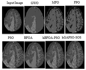
5.3 Qualitative analysis
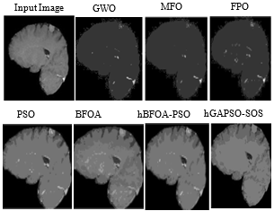
Here we focus on visual clarity of decompressed images with the proposed work by maximizing the Renyi entropy by thresholding the image with proposed hybrid GAPSO-SOS and with GWO, MFO, FPO, PSO, BFOA and hBFOA-PSO algorithms. Figure 10 to Figure 15 below, shows original MRI brain images and the corresponding decompressed images of GWO, MFO, FPO, PSO, BFOA, hBFOA-PSO and hybrid GAPSO-SOS algorithms of Astrocytoma, Coronary T1 Astrocytoma, Glioma, Metastatic, PNET, and Meningioma brain MRI images respectively.
Table 3. Performance evaluation of PSNR & MSE values of seven algorithms for brain images
|
Brain Input Images |
Optimization Technique |
PSNR in dB |
MSE |
||
|
1-D histogram |
2-D histogram |
1-D histogram |
2-D histogram |
||
|
Meningioma |
GWO |
36.36813 |
36.54231 |
17.6145 |
16.3126 |
|
MFO |
36.46615 |
36.64134 |
15.5373 |
14.2353 |
|
|
FPO |
36.54133 |
36.79182 |
14.7675 |
13.3815 |
|
|
PSO |
36.84133 |
36.88658 |
13.4569 |
13.31749 |
|
|
BFOA |
37.39621 |
37.47584 |
11.8429 |
11.62777 |
|
|
hBFOA-PSO |
37.58954 |
38.65026 |
11.3273 |
8.872671 |
|
|
hGAPSO-SOS |
39.10687 |
39.91545 |
7.9871 |
7.789962 |
|
|
PNET |
GWO |
34.26407 |
34.66402 |
18.8179 |
18.8179 |
|
MFO |
34.55097 |
35.05037 |
17.6144 |
17.6144 |
|
|
FPO |
34.78454 |
35.53424 |
16.2546 |
14.2641 |
|
|
PSO |
35.09575 |
35.99365 |
15.5373 |
13.2343 |
|
|
BFOA |
35.31654 |
36.21428 |
14.7672 |
13.1532 |
|
|
hBFOA-PSO |
35.55442 |
37.16502 |
13.9807 |
11.6745 |
|
|
hGAPSO-SOS |
36.54231 |
38.38712 |
11.5923 |
9.7609 |
|
|
Metastatic |
GWO |
29.12323 |
29.72544 |
61.4678 |
53.6106 |
|
MFO |
29.21606 |
30.16525 |
60.1674 |
48.8914 |
|
|
FPO |
29.23780 |
30.29682 |
59.8663 |
48.2973 |
|
|
PSO |
29.29132 |
31.26530 |
59.1335 |
47.1272 |
|
|
BFOA |
29.72694 |
31.15134 |
53.4896 |
43.7657 |
|
|
hBFOA-PSO |
31.96948 |
32.95464 |
31.9162 |
28.6059 |
|
|
hGAPSO-SOS |
32.27554 |
33.79839 |
29.7458 |
19.8202 |
|
|
Glioma |
GWO |
28.92734 |
29.72694 |
56.3952 |
53.489 |
|
MFO |
29.18506 |
30.16053 |
37.6738 |
38.891 |
|
|
FPO |
31.96948 |
32.52526 |
31.9169 |
28.605 |
|
|
PSO |
32.27554 |
32.86587 |
38.50582 |
37.7132 |
|
|
BFOA |
32.84134 |
32.98745 |
33.80231 |
32.68401 |
|
|
hBFOA-PSO |
33.04264 |
34.25874 |
32.27129 |
30.70481 |
|
|
hGAPSO-SOS |
33.83699 |
34.90258 |
26.87704 |
26.47417 |
|
|
Coronary T1Astrocytoma |
GWO |
33.04206 |
33.5691 |
32.24120 |
27.02921 |
|
MFO |
33.66409 |
33.9583 |
30.71342 |
25.16091 |
|
|
FPO |
33.75482 |
33.9987 |
28.90347 |
23.18384 |
|
|
PSO |
33.77889 |
33.96724 |
27.23901 |
22.3451 |
|
|
BFOA |
34.00706 |
34.43670 |
25.84487 |
21.6054 |
|
|
hBFOA-PSO |
34.35888 |
34.97895 |
23.83375 |
21.1582 |
|
|
hGAPSO-SOS |
34.56214 |
35.96587 |
22.74397 |
20.72494 |
|
|
Astrocytoma |
GWO |
30.34729 |
31.969481 |
46.369 |
31.916 |
|
MFO |
32.54134 |
32.855644 |
27.978 |
26.025 |
|
|
FPO |
32.74866 |
33.042064 |
26.675 |
24.932 |
|
|
PSO |
34.03859 |
34.25874 |
25.65791 |
24.38969 |
|
|
BFOA |
35.00920 |
35.33568 |
20.5192 |
19.03322 |
|
|
hBFOA-PSO |
35.08465 |
35.45789 |
20.1658 |
18.5051 |
|
|
hGAPSO-SOS |
35.29112 |
35.65894 |
19.22952 |
17.66796 |
|
Figure 10. Decompressed images obtained with seven algorithms of Astrocytoma brain image
Figure 11. Decompressed images obtained with seven algorithms of Coronary T1 Astrocytoma brain image
Table 4. Comparison of WPSNR, VPSNR and Elapsed time values of brain images for various algorithms
|
Brain Input Images |
Optimization Technique |
WPSNR in dB |
VPSNR in dB |
Elapsed time (sec) |
|||
|
1-D histogram |
2-D histogram |
1-D histogram |
2-D histogram |
1-D histogram |
2-D histogram |
||
|
Meningioma |
GWO |
15.6090 |
15.847 |
15.079 |
15.278 |
10.781 |
9.284 |
|
MFO |
15.8353 |
16.189 |
15.134 |
15.375 |
7.238 |
6.013 |
|
|
FPO |
15.9374 |
16.492 |
15.198 |
15.483 |
12.435 |
11.364 |
|
|
PSO |
16.0525 |
16.768 |
15.256 |
15.568 |
9.224 |
7.782 |
|
|
BFOA |
18.1255 |
18.978 |
16.124 |
16.258 |
7.020 |
5.567 |
|
|
hBFOA-PSO |
19.0003 |
20.024 |
17.102 |
17.478 |
57.999 |
49.24 |
|
|
hGAPSO-SOS |
19.7084 |
20.147 |
19.258 |
19.985 |
64.345 |
54.421 |
|
|
PNET |
GWO |
18.1534 |
18.345 |
15.264 |
15.583 |
16.912 |
14.957 |
|
MFO |
18.5318 |
18.675 |
15.459 |
15.954 |
7.173 |
6.023 |
|
|
FPO |
18.7523 |
18.967 |
15.973 |
16.367 |
17.234 |
15.024 |
|
|
PSO |
18.9432 |
19.198 |
16.247 |
16.756 |
9.805 |
7.643 |
|
|
BFOA |
19.0816 |
19.543 |
16.725 |
17.034 |
7.602 |
6.104 |
|
|
hBFOA-PSO |
20.2464 |
20.349 |
17.246 |
17.746 |
59.418 |
45.375 |
|
|
hGAPSO-SOS |
20.7398 |
20.986 |
18.027 |
18.958 |
71.348 |
58.426 |
|
|
Metastatic |
GWO |
25.6666 |
25.813 |
16.323 |
16.575 |
15.427 |
13.765 |
|
MFO |
25.7612 |
25.985 |
16.785 |
16.983 |
10.716 |
8.342 |
|
|
FPO |
25.9765 |
26.078 |
17.253 |
17.859 |
14.274 |
12.869 |
|
|
PSO |
26.4718 |
26.654 |
17.648 |
18.023 |
8.235 |
6.234 |
|
|
BFOA |
26.4960 |
26.942 |
17.904 |
18.867 |
9.443 |
7.569 |
|
|
hBFOA-PSO |
26.5009 |
26.875 |
18.127 |
18.849 |
48.395 |
36.235 |
|
|
hGAPSO-SOS |
26.7258 |
27.362 |
18.984 |
19.694 |
59.142 |
43.654 |
|
|
Glioma |
GWO |
16.9745 |
17.324 |
14.042 |
14.234 |
12.145 |
11.570 |
|
MFO |
17.6191 |
17.976 |
14.197 |
14.769 |
7.867 |
5.635 |
|
|
FPO |
18.2012 |
18.574 |
14.326 |
15.168 |
15.562 |
13.794 |
|
|
PSO |
18.7953 |
18.987 |
14.457 |
16.909 |
9.9885 |
6.270 |
|
|
BFOA |
18.9130 |
18.978 |
14.698 |
18.024 |
17.692 |
12.781 |
|
|
hBFOA-PSO |
19.1240 |
19.057 |
16.457 |
18.245 |
52.848 |
46.251 |
|
|
hGAPSO-SOS |
19.2351 |
19.333 |
19.985 |
19.658 |
71.753 |
63.231 |
|
|
Coronary T1 Astrocytoma |
GWO |
17.6281 |
17.874 |
15.109 |
15.367 |
16.924 |
14.768 |
|
MFO |
17.8520 |
17.924 |
15.298 |
15.896 |
9.041 |
7.325 |
|
|
FPO |
17.905 |
18.016 |
15.567 |
16.638 |
15.835 |
13.573 |
|
|
PSO |
18.1561 |
18.245 |
16.102 |
18.214 |
10.561 |
7.529 |
|
|
BFOA |
19.9524 |
19.447 |
16.247 |
19.247 |
8.3687 |
5.321 |
|
|
hBFOA-PSO |
20.5253 |
20.727 |
16.367 |
22.124 |
58.186 |
51.982 |
|
|
hGAPSO-SOS |
20.8112 |
20.963 |
18.247 |
22.247 |
74.386 |
64.342 |
|
|
Astrocytoma |
GWO |
17.0790 |
17.354 |
16.018 |
16.675 |
21.726 |
20.047 |
|
MFO |
17.6321 |
17.860 |
16.249 |
17.028 |
8.054 |
6.958 |
|
|
FPO |
18.7072 |
18.864 |
16.573 |
17.893 |
16.392 |
14.538 |
|
|
PSO |
18.8089 |
18.947 |
16.957 |
18.608 |
13.634 |
9.527 |
|
|
BFOA |
19.5862 |
19.658 |
17.547 |
18.425 |
7.9109 |
4.632 |
|
|
hBFOA-PSO |
19.8229 |
19.919 |
18.654 |
19.962 |
65.194 |
56.036 |
|
|
hGAPSO-SOS |
20.1235 |
20.207 |
19.102 |
20.753 |
83.561 |
74.375 |
|
Figure 12. Decompressed images obtained with seven algorithms of Glioma brain image
Figure 13. Decompressed images obtained with seven algorithms of Metastatic brain image
Table 5. Evaluation of BPP and CR of seven algorithms for brain images
|
Image |
Optimization Technique |
BPPcode |
CRcode |
||
|
1-D |
2-D |
1-D |
2-D |
||
|
Meningioma |
GWO |
0.2787556 |
0.5971753 |
28.69898 |
13.396401 |
|
MFO |
0.2686425 |
0.5900642 |
29.779412 |
13.557847 |
|
|
FPO |
0.3159341 |
0.5950264 |
25.323712 |
13.443581 |
|
|
PSO |
0.3038815 |
0.7379753 |
26.326053 |
10.840471 |
|
|
BFOA |
0.2710123 |
0.6313086 |
29.51895 |
12.67209 |
|
|
HBFOA-PSO |
0.2785975 |
0.6992593 |
28.715258 |
11.440678 |
|
|
hGAPSO-SOS |
0.2644136 |
0.5981274 |
30.252436 |
13.371352 |
|
|
PNET |
GWO |
0.4979358 |
0.8427457 |
16.066328 |
8.4024896 |
|
MFO |
0.5513481 |
0.895842 |
14.509888 |
8.9301464 |
|
|
FPO |
0.5596457 |
0.8709453 |
14.296814 |
9.1857568 |
|
|
PSO |
0.4998321 |
0.9520988 |
16.005375 |
9.1150522 |
|
|
BFOA |
0.537758 |
0.8776691 |
14.876579 |
9.4927808 |
|
|
HBFOA-PSO |
0.4984099 |
0.7341827 |
16.051046 |
10.896478 |
|
|
hGAPSO-SOS |
0.4331901 |
0.6019214 |
18.474372 |
13.292636 |
|
|
Metastatic |
GWO |
0.6842469 |
0.9438815 |
11.691686 |
8.4756404 |
|
MFO |
0.7204346 |
0.9636346 |
11.104409 |
8.3019023 |
|
|
FPO |
0.6060241 |
0.872634 |
13.198095 |
9.1673452 |
|
|
PSO |
0.6844049 |
0.8918914 |
11.688986 |
8.9697023 |
|
|
BFOA |
0.6902519 |
0.9440395 |
11.589973 |
8.4742216 |
|
|
HBFOA-PSO |
0.8124049 |
0.8564938 |
9.847306 |
9.3404059 |
|
|
hGAPSO-SOS |
0.8557365 |
0.8907356 |
9.3482158 |
8.9816747 |
|
|
Glioma |
GWO |
0.691358 |
0.8351605 |
11.571429 |
9.5789972 |
|
MFO |
0.7659457 |
0.9770667 |
10.444605 |
8.1877729 |
|
|
FPO |
0.5596234 |
0.8557345 |
14.293127 |
9.3482134 |
|
|
PSO |
0.5627259 |
0.857916 |
14.216512 |
9.3249217 |
|
|
BFOA |
0.7651556 |
1.0140444 |
10.45539 |
7.8892006 |
|
|
HBFOA-PSO |
0.5619358 |
0.9034272 |
14.236502 |
8.8551688 |
|
|
hGAPSO-SOS |
0.5596236 |
0.8842670 |
14.293267 |
9.0465673 |
|
|
Coronary T1 Astrocytoma |
GWO |
0.5456593 |
0.5652543 |
14.661164 |
14.152921 |
|
MFO |
0.5864296 |
0.5508741 |
13.641876 |
14.522375 |
|
|
FPO |
0.4295543 |
0.5950232 |
18.626792 |
13.442674 |
|
|
PSO |
0.3318519 |
0.6363654 |
24.107143 |
12.571393 |
|
|
BFOA |
0.5897481 |
0.5357037 |
13.565113 |
14.933628 |
|
|
HBFOA-PSO |
0.5347556 |
0.7085827 |
14.960106 |
11.290143 |
|
|
hGAPSO-SOS |
0.5981890 |
0.5972342 |
13.375672 |
13.395672 |
|
|
Astrocytoma |
GWO |
0.5684148 |
0.7841185 |
14.074229 |
10.202539 |
|
MFO |
0.5420247 |
0.8209383 |
14.759475 |
9.7449471 |
|
|
FPO |
0.4295123 |
0.8624356 |
18.626793 |
9.2763452 |
|
|
PSO |
0.3373827 |
0.8267852 |
23.711944 |
9.6760321 |
|
|
BFOA |
0.5564049 |
0.5782123 |
14.378018 |
13.835747 |
|
|
HBFOA-PSO |
0.557037 |
0.5515062 |
14.361702 |
14.505731 |
|
|
hGAPSO-SOS |
0.611978 |
0.6018234 |
13.074367 |
13.294563 |
|
Figure 14. Decompressed images obtained with seven algorithms of PNET brain image
Figure 15. Decompressed images obtained with seven algorithms of Meningioma brain image
From figures, it is seen that decompressed image quality of the proposed hGAPSO-SOS is better than the other individual algorithms.
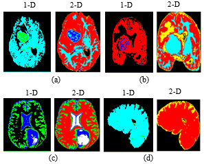
Figure 16. Decompressed images of hGAPSO-SOS algorithm with 1-D and 2-D histogram: (a) Astrocytoma (b) Coronary (c) Glioma (d) Meningioma
For efficiency measure of proposed algorithm hybrid GAPSO-SOS, the visual quality of reconstructed images has to be evaluated in Figure 16 a-d with Renyi entropy at five number of thresholds in 1-D and proposed 2-D histogram. From the figures, it is seen that hGAPSO-SOS visual quality is better for 2-D histogram as related to 1-D histogram.
In this paper, Hybridization of Genetic Algorithm, Particle Swarm Optimization and Symbiotic Organisms Search is used for decisive and efficient multilevel thresholding for image compression. Optimal threshold values are provided by maximizing the Renyi entropy using 2-D histogram which leads to better image thresholding. So, meaningful/useful clusters are possible with optimal threshold values, leads to better image compression. For performance evaluation, the proposed hGAPSO-SOS algorithm is tested on six MR brain images. Performance of proposed 2-D histogram thresholding technique is validated with performance metrics of fitness function, MSE, PSNR, CR, WPSNR, and, VPSNR. The procured result of the hGAPSO-SOS is compared with other optimization algorithms such as GWO, MFO, FPO, PSO, BFOA and hBFOA-PSO. From comparison, it is observed that hGAPSO-SOS algorithm provides better fitness value, higher PSNR, VPSNR, WPSNR values and maintain good quality of the reconstructed images with better CR than other six algorithms. From the results, it is concluded that the Hybridization of optimization algorithms enhances all performance parameters than other individual algorithms and also found to be better with 2-D than with the 1-D histogram. From results, it shows that proposed hGAPSO-SOS method is more reliable than GWO, MFO, FPO, PSO, BFOA and hBFOA-PSO and, can be efficiently used in problem of multilevel thresholding for medical image compression.
[1] Pennebaker, W.B., Mitchell, J.L. (1992). JPEG: Still Image Data Compression Standard. Springer Science & Business Media.
[2] Ahmed, N., Natarajan, T., Rao, K.R. (1974). Discrete cosine transform. IEEE Transactions on Computers, 100(1): 90-93. https://doi.org/10.1109/T-C.1974.223784
[3] DeVore, R.A., Jawerth, B., Lucier, B.J. (1992). Image compression through wavelet transform coding. IEEE Transactions on Information Theory, 38(2): 719-746. https://doi.org/10.1109/18.119733
[4] Acharya, T., Tsai, P.S. (2005). JPEG2000 Standard for Image Compression: Concepts, Algorithms and VLSI Architectures. John Wiley & Sons. https://doi.org/10.1002/0471653748.ch6
[5] Skodras, A.N., Christopoulos, C.A., Ebrahimi, T. (2001). JPEG2000: The upcoming still image compression standard. Pattern Recognition Letters, 22(12): 1337-1345. https://doi.org/10.1016/S0167-8655(01)00079-4
[6] Santa-Cruz, D., Ebrahimi, T. (2000). An analytical study of JPEG 2000 functionalities. In Proceedings 2000 International Conference on Image Processing (Cat. No. 00CH37101), 2: 49-52. https://doi.org/10.1109/ICIP.2000.899222
[7] De, A., Guo, C. (2015). An adaptive vector quantization approach for image segmentation based on SOM network. Neurocomputing, 149: 48-58. https://doi.org/10.1016/j.neucom.2014.02.069
[8] Linde, Y., Buzo, A., Gray, R. (1980). An algorithm for vector quantizer design. IEEE Transactions on Communications, 28(1): 84-95. https://doi.org/10.1109/TCOM.1980.1094577
[9] Rajpoot, N.M., Hussain, A., Ali, U., Saleem, K., Qureshi, M. (2004). A novel image coding algorithm using ant colony system vector quantization. In: International Workshop on Systems, Signals and Image Processing (IWSSIP 2004), Poznan, Poland, pp. 13-15.
[10] Kumar, M., Kapoor, R., Goel, T. (2010). Vector quantization based on self-adaptive particle swarm optimization. International Journal of Nonlinear Sciences, 9(3): 311-319.
[11] Wang, Y., Feng, X.Y., Huang, Y.X., Pu, D.B., Zhou, W.G., Liang, Y.C., Zhou, C.G. (2007). A novel quantum swarm evolutionary algorithm and its applications. Neurocomputing, 70(4-6): 633-640. https://doi.org/10.1016/j.neucom.2006.10.001
[12] Kumari, G.V., Rao, G.S., Rao, B.P. (2021). Flower pollination-based K-means algorithm for medical image compression. International Journal of Advanced Intelligence Paradigms, 18(2): 171-192. https://doi.org/10.1504/IJAIP.2021.112903
[13] Chiranjeevi, K., Jena, U. (2017). Hybrid gravitational search and pattern search–based image thresholding by optimising Shannon and fuzzy entropy for image compression. International Journal of Image and Data Fusion, 8(3): 236-269. https://doi.org/10.1080/19479832.2017.1338760
[14] Sheeba, K., Rahiman, M.A. (2019). Gradient based fractal image compression using Cayley table. Measurement, 140: 126-132. https://doi.org/10.1016/j.measurement.2019.02.038
[15] Patel, B., Agrawal, S. (2013). Image compression techniques using artificial neural network. International Journal of Advanced Research in Computer Engineering & Technology, 2(10): 2725-2729.
[16] Kumari, G.V., Rao, G.S., Rao, B.P. (2019). New artificial neural network models for bio medical image compression: bio medical image compression. International Journal of Applied Metaheuristic Computing (IJAMC), 10(4): 91-111. https://doi.org/10.4018/IJAMC.2019100106
[17] Mardani, M., Gong, E., Cheng, J.Y., Vasanawala, S.S., Zaharchuk, G., Xing, L., Pauly, J.M. (2018). Deep generative adversarial neural networks for compressive sensing MRI. IEEE Transactions on Medical Imaging, 38(1): 167-179. https://doi.org/10.1109/TMI.2018.2858752
[18] Gözcü, B., Mahabadi, R.K., Li, Y.H., Ilıcak, E., Cukur, T., Scarlett, J., Cevher, V. (2018). Learning-based compressive MRI. IEEE Transactions on Medical Imaging, 37(6): 1394-1406. https://doi.org/10.1109/TMI.2018.2832540
[19] Gao, S., Xiong, Z. (2019). Deep enhancement for 3D HDR brain image compression. In 2019 IEEE International Conference on Image Processing (ICIP), pp. 714-718. https://doi.org/10.1109/ICIP.2019.8803781
[20] De Luca, A., Termini, S. (1972). A definition of a nonprobabilistic entropy in the setting of fuzzy sets theory. Information and Control, 20(4): 301-312. https://doi.org/10.1016/S0019-9958(72)90199-4
[21] Tryon, R.C. (2016). Cluster analysis: correlation profile and ortho-metric (factor) analysis for the isolation of unities in mind and personality. Applied Mathematics, 7(15): 231-239.
[22] Sidhik, S. (2015). Comparative study of Birge–Massart strategy and unimodal thresholding for image compression using wavelet transform. Optik, 126(24): 5952-5955. https://doi.org/10.1016/j.ijleo.2015.08.127
[23] Adhikari, S.K., Sing, J.K., Basu, D.K., Nasipuri, M. (2015). Conditional spatial fuzzy C-means clustering algorithm for segmentation of MRI images. Applied Soft Computing, 34: 758-769. https://doi.org/10.1016/j.asoc.2015.05.038
[24] Ramakrishnan, T., Sankaragomathi, B. (2017). A professional estimate on the computed tomography brain tumor images using SVM-SMO for classification and MRG-GWO for segmentation. Pattern Recognition Letters, 94: 163-171. https://doi.org/10.1016/j.patrec.2017.03.026
[25] Salleh, M.F.M., Soraghan, J. (2007). A new multistage lattice vector quantization with adaptive subband thresholding for image compression. EURASIP Journal on Advances in Signal Processing, 2007: 1-11. https://doi.org/10.1155/2007/92928
[26] De Albuquerque, M.P., Esquef, I.A., Mello, A.G. (2004). Image thresholding using Tsallis entropy. Pattern Recognition Letters, 25(9): 1059-1065. https://doi.org/10.1016/j.patrec.2004.03.003
[27] Kumari, G.V., Rao, G.S., Rao, B.P. (2018). New bacteria foraging and particle swarm hybrid algorithm for medical image compression. Image Analysis & Stereology, 37(3): 249-275. https://doi.org/10.5566/ias.1865
[28] Ahilan, A., Manogaran, G., Raja, C., Kadry, S., Kumar, S.N., Kumar, C.A., Murugan, N.S. (2019). Segmentation by fractional order Darwinian particle swarm optimization based multilevel thresholding and improved lossless prediction based compression algorithm for medical images. IEEE Access, 7: 89570-89580. https://doi.org/10.1109/ACCESS.2019.2891632
[29] Hoang, T.M., Zhou, J., Fan, Y. (2020). Image compression with encoder-decoder matched semantic segmentation. 2020 IEEE/CVF Conference on Computer Vision and Pattern Recognition Workshops (CVPRW), pp. 619-623. https://doi.org/10.1109/CVPRW50498.2020.00088
[30] Sarkar, S., Das, S. (2013). Multilevel image thresholding based on 2D histogram and maximum Tsallis entropy—a differential evolution approach. IEEE Transactions on Image Processing, 22(12): 4788-4797. https://doi.org/10.1109/TIP.2013.2277832
[31] Farnad, B., Jafarian, A., Baleanu, D. (2018). A new hybrid algorithm for continuous optimization problem. Applied Mathematical Modelling, 55: 652-673. https://doi.org/10.1016/j.apm.2017.10.001