Menaka Radhakrishnan* | Karthik Ramamurthy | Kaustav Kumar Choudhury | Daehan Won | Thanga Aarthy Manoharan
© 2021 IIETA. This article is published by IIETA and is licensed under the CC BY 4.0 license (http://creativecommons.org/licenses/by/4.0/).
OPEN ACCESS
Autism Spectrum Disorder (ASD) starts showing symptoms in the early formative years of an individual, affecting brain development and negatively impacting social and communication skills. Subjective diagnostic methods for ASD detection require lengthy questionnaires, trained medical personnel, and occupational therapists, and are subject to observer variability. Recent years have seen a rise in the usage of machine learning techniques for detecting ASD, which stems from a requirement for objective and accurate detection methods. This research analyzes the performance of various deep convolutional architectures for the detection of ASD. The primary objective of this work is to select a method capable of performing automatic feature extraction and classification with a relatively high degree of accuracy. Several experiments were conducted with different state-of-the-art deep architectures, out of which the ResNet50 performed the best, with an average accuracy of 81%. The performances of these architectures were analyzed in terms of precision, recall, and accuracy.
ASD, EEG, spectrogram, deep learning, CNN, accuracy
Autism Spectrum Disorder (ASD) can be defined as a set of neurodevelopmental disorders, primarily characterized by a deficit in social behavior and non-verbal interactions [1]. It includes reduced eye contact, facial expressions, and body gestures in the first three years of life. The disorder starts manifesting during early childhood and lasts a lifetime. The Morbidity and Mortality Weekly Report (MMWR) by CDC stated that as of 2014, 1 in every 59 children aged 8 years was autistic, based on the data obtained from different sites in the USA [2]. The ‘spectrum’ in ASD is for indicating that autistic individuals can have a multitude of symptoms. Such symptoms include obsession with arranging things, repeating the same words or sentences multiple times, and struggling to achieve meaningful social interaction. Individuals diagnosed with ASD also have high rates of anxiety disorders, as indicated by the data collected from epidemiological and clinical samples [3].
The Centers for Disease Control and Prevention states that autism is more likely to affect males as compared to females. There is a 4-to-1 male-to-female ratio in occurrences of autism. The Diagnostic and Statistic Manual of Mental Disorders (DSM), published by the American Psychiatric Association (APA), is used to diagnose various mental disorders. In 2013, the most recent edition of the DSM was released, which recognizes five different ASD sub-types [4].
There are a variety of tests that can be used to determine whether a child is autistic or not. These include, but are not limited to, behavioral evaluation and occupational therapy screening. Some of the more popular clinical methods are Childhood Autism Rating Scale (CARS), Autism Diagnostic Observation Schedule (ADOS), Autism Diagnostic Interview-Revised (ADI-R), and the social responsiveness scale. However, each of these methods has its advantages and its shortcomings. They are time-consuming, have long questionnaires, and require certified professionals for administration [5].
Brain waves are created when masses of neurons receive inputs together. These waves are then picked up as electrical signals through an EEG [6]. Brainwaves carry various types of rhythms that are reflective of several different types of information [7, 8]. Welsh and Estes [9] observed that the flow of information in the brains of autistic children during social processing was different than normal controls. Another observation by them was that all changes in information flow in the brain were not maladaptive [9]. Thus, the features of the EEG signals obtained from an autistic child may not have any discernible differences as compared with a normal child. This research work attempts to apply automatic feature extraction and learning for ASD detection from EEG signals.
Conventional methods of detecting autism are primarily focused on observational techniques and cognitive assessments. Observational assessments include focused observations taken across more than one setting (such as home, nursery, etc.) [10]. There has been a lot of progress in recent years in the use of both machine learning and deep learning for the detection of autism.
2.1 Machine learning-based methods
Machine learning (ML) is a sub-class of Artificial Intelligence, where systems learn from experience without being directly programmed as such. ML is used to formulate different complex modes to make accurate classifications/predictions on different types of data [11]. Methods like Support Vector Machine (SVM) [12], decision tree [13], and random forest [14] have already been tried and tested for detecting autism [15].
Grether et al. [16] used logistic regression to determine the impact of parental age as a contributing factor to the development of autism in their offspring. Other than evaluating risk factors, logistic regression has also been used for neuro-imaging and classification. Plitt et al. [17] used logistic regression to determine the significance of rs-fMRI scans in detecting ASD biomarkers. Duda et al. [18] used Support Vector Classification, Categorical Lasso and Logistic Regression to distinguish between ASD and ADHD EEG signals. Chen et al. [19] used Support Vector Machine (SVM) in combination with particle swarm optimization (PSO) for feature selection, SVM with recursive feature elimination (RFE-SVM) for feature ranking, and Random Forest for classifying ASD EEG-signals. Data from Autism Brain Imaging Data Exchange (ABIDE) was used in this research, which is a collection of over 1100 resting-state scans from 17 different sites. Boutros et al. [20] used Quantitative EEG (qEEG) for assessing 17 autistic and 11 non-autistic children. Quantitative EEG was also recommended by Sheikhani et al. [21] as an approach to the classification of EEG signals. In qEEG, the EEG activity is recorded by a multi-electrode device and is processed using various algorithms like Fourier or Wavelet analysis. This data is then analyzed statistically and converted into “brain maps” to indicate the functioning aspect of the brain.
The analysis of spectral features of an EEG signal using machine learning has also been carried out previously. Choe et al. (2010) extracted the power spectral density from EEG signals, using the multi-taper method for estimation, combined with Linear Discriminant Analysis (LDA) [22]. Bascil et al. (2016) extracted the power spectral density (PSD) from EEG signals and used least squares SVM (LS-SVM) and Artificial Neural Networks to carry out pattern recognition during mental tasks of 2-D cursor movements [23]. Tsipouras (2019) worked on the detection of epilepsy from EEG signals using spectral feature extraction and analysis [24]. The impact of the frequency sub-bands on EEG classification accuracy was analyzed.
Other than using the statistical and spectral features of EEG signals, non-linear features like Recurrence Quantification Analysis (RQA) have also been used for the classification of EEG signals. Acharya et al. [25] extracted RQA parameters from Recurrence Plots to classify the obtained EEG signals into normal, ictal, and interictal classes, for the automatic identification of epileptic EEG signals. Heunis et al. (2018) assessed the robustness of RQA as a potential biomarker for ASD. The authors stated that the RQA of rsEEG was an accurate classifier of ASD [26]. However, this study also showed that a range of technical and demographic challenges could skew the results. Bosl et al. [27] computed the multiscale entropy and multiscale version of RQA obtained from EEG data and made statistical comparisons to find neurophysiological differences between autism and absence epilepsy. Machine learning models were used to estimate the significance of the derived features and to calculate classification specificity and sensitivity.
Using machine learning methods has offered good solutions, as evidenced by the works listed above. However, the usage of deep neural networks has an inherent advantage over machine learning. Deep learning is equipped to execute feature engineering autonomously, whereas machine learning requires manual feature extraction. This flexibility offered in terms of feature extraction gives deep learning an edge over machine learning when dealing with diverse datasets. Furthermore, deep learning models offer much better performance metrics when dealing with unstructured data. Thus, deep learning has many advantages over machine learning.
2.2 Deep learning-based methods
Deep learning, a sub-class of machine learning, uses several non-linear layers of information processing for supervised or unsupervised extraction of features, transformation, pattern analysis, and classification [28]. Tabar and Halici [29] showed that CNNs and Stacked Auto-encoder networks (SAE) [30], i.e. a deep learning approach, gave better results as compared to traditional machine learning algorithms for EEG signal processing and classification. CNNs are capable of performing automatic feature extraction, which eliminates the need for a more detailed manual feature analysis.
One-dimensional Convolutional Neural Networks (1D CNNs) have been used previously for the classification of EEG signals. Yıldırım et al. (2018) proposed an end-to-end system for the classification of EEG signals without any manual feature extraction using 1D CNN [31]. Zabihi et al. [32] investigated the efficiency of five different 1D CNN architectures and performed comparative evaluations to determine the best model for classification. Although 1D CNNs offered promising results in classifying EEG signals, Wu et al. [33] observed that 2D CNNs offer better results for EEG signals. Compared with signal input methods in 1D-CNNs, 2D-CNNs can perform fine-tuning with large databases, achieving higher accuracy and robustness. Moreover, the Imagenet-2D architecture achieved an accuracy of 98%, while the Swish-1D architecture achieved an accuracy of 96%. Thus, 2D CNNs have a clear advantage over 1D CNNs.
Liu et al. [34] used 2D CNN architectures to model the consciousness levels of patients under the effect of anesthetics by plotting spectrograms of the EEG signals. Kwon et al. [35] studied the EEG signals obtained from the frontal lobe, which was then used to model an emotion recognition system using 2D CNN architectures. Ozdemir et al. [36] proposed an approach for emotional state estimation using 2D CNN architectures, applied to EEG signals. The EEG signals were converted to 2D EEG images with Azimuthal Equidistant Projection (AEP) technique. Then, two-dimensional images that represent EEG signal measurements were fed to a CNN-based deep network for classification.
Multiple approaches and architectures were presented for the detection of ASD from brain EEG signals in the last two decades. However, it is not possible to replicate the results obtained using the same architectures on different datasets. This gives rise to a need for analyzing the evaluation metrics for many different models to obtain the most suitable architecture for a given dataset.
2.3 Research gap and motivation
Though different approaches were developed for ASD detection in the past two decades, there exist some potential challenges in it.
1. The methods of diagnosing autism primarily consist of clinical diagnostic processes. As mentioned previously, some of the more popular clinical methods for detecting autism are Autism Diagnostic Interview-Revised (ADI-R) and Autism Diagnostic Observation Schedule (ADOS). These methods have long questionnaires and require certified medical personnel for administration. These subjective assessment techniques are usually prone to inter and intra-observer variability. Thus, a more streamlined and objective method is required.
2. The methods for detecting autism using machine learning techniques are heavily reliant on the availability and/or extraction of handcrafted features. As these methods use EEG signals for classification, procuring handcrafted features is not always a feasible solution.
Considering the above-mentioned points, the following key challenges are addressed in this work.
3. A fully automated approach to extract key features from EEG signals, and subsequently using those features for classification is needed. This task can be accomplished with the help of deep 2D convolutional networks.
4. Since deep convolutional networks are fully equipped to perform automatic feature extraction, and the performance of deep networks typically depends on the nature of the underlying architecture, many different deep architectures have been compared and contrasted against each other in this work.
2.4 Research contribution
The key contributions of this research are reported as follows:
1. The proposed research has performed a comprehensive analysis with state-of-the-art deep architectures for ASD detection. CNN-based models like AlexNet, DenseNet, SqueezeNet, ShuffleNet, VGGNet, InceptionNet, and ResNet were analyzed based on different performance metrics.
2. To the best of our knowledge, this is the first report which compares the performance of different state-of-the-art deep architectures for Autism detection. Although many articles have employed transfer learning with one or two networks, there exists a vital need to compare the performance of all networks under a unified computing setting. This will help us to identify a suitable architecture that could model the intrinsic characteristics of Autistic EEG signals in a better way.
3. After evaluating performance metrics like Specificity and F1-score for many models, ResNet50 was observed to give the best results on k-fold cross-validation. Hence, a deep architecture using ResNet50 was then proposed for the detection of ASD from EEG signals.
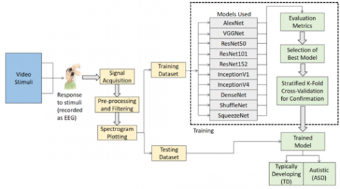
An overview of the proposed system is presented in Figure 1.
3.1 Data acquisition
The parents/guardians of the participants involved in this study were advised to refer to and sign a consent form. The study protocol was based on the manual “Helsinki Ethical Principles and ICMR Ethical Guidelines” [37]. The EEG data were collected from 10 typically developing children (6 Male and 6 Female) and 10 autistic children (6 Male and 4 Female).
EEG records were collected from an acquisition system with the following specifications: Natus Nihon Ohden MEB9000 version 05-81, with a sensitivity of 7 microvolts. The data acquisition was performed using International 10-20 electrode systems, as presented in Figure 2. The 10-20 systems divide the scalp into six different regions namely: Frontopolar (Fp), Frontal(F), Temporal(T), Parietal(P), Occipital(O), Central(C), Ear Lobe(A). Each of these regions is responsible for a particular activity, and is activated based on the stimulus given.
The subjects were seated in a room with standard lighting and low noise. The distance between the subject’s eye and the 32” monitor was 50±5 cm, depending on the height of the subject. The Ag/Agcl electrodes were then positioned on the subject’s scalp using conductive gel and tapes. The subjects were made to watch an animated video for 10 minutes.
Figure 1. Overview of the proposed system
Figure 2. 10-20 electrode positioning pattern
3.2 Pre-processing
The EEG signals were recorded from 22 channels with a sampling frequency of 500 Hz and filtered with a low pass filter and a high pass filter at a frequency range of [0.53-70 Hz]. After filtering out the signal at a frequency range of 0.53 to 70 Hz, the ocular artifacts in the EEG signal were removed by thresholding. The threshold was set based on the average value of the amplitude of the eye blink signal. The eye blink signal was observed for 10 seconds with the eye open and eye close event. After thresholding, the resultant signal was further considered for analysis.
3.3 Spectrogram plotting
A spectrogram is a visual representation of the strength or the “loudness” of a signal. The colors of the spectrogram and their brightness indicate the signal strength: the brighter the color, the higher the strength of the signal. A spectrogram plots frequencies on X-axis and time on Y-axis. For plotting the spectrogram of a signal, it is divided into short segments of equal lengths, such that the frequency does not change significantly over time in each segment. Then a Discrete Fourier Transform (DFT) is applied to each segment. A succession of these DFTs is then used to calculate the Short-Time Fourier Transform.
A Short-Time Fourier Transform, or STFT, is used to calculate sinusoidal frequency and determine the phase content of a signal ‘x(n)’ that has been divided into sections, as the signal changes over time. The relation for STFT is presented in Eq. (1).
$Xm(\omega )=\,\sum\limits_{n=-\infty }^{\infty }{x(n)w(n)e\begin{matrix} -j\omega n \\ {} \\\end{matrix}}$ (1)
where,
Xm(ω) = DTFT of the given signal
x(n) = input signal at time n
w(n) = windowing function
The STFT is then calculated as per the relation presented in Eq. (2).
$STFT\,=\,DTFT(x\cdot SHIFTmR(w))$ (2)
where,
R=hop size between successive DTFTs, measured in samples.
m=index of the windowed block of the signal x(n).
The multi-channel signals were reshaped into 1-dimensional arrays, which were then used to plot the spectrograms. From an implementation point of view, the STFT is calculated as a succession of FFTs of windowed data frames, where the window slides forward through time. The relation for the STFT is then slightly modified, by adding the ‘mR’ term to ‘n’, and given as per Eq. (3).
$Xm(\omega )=\,\sum\limits_{n=-\infty }^{\infty }{x(n+mR)w(n)e\begin{matrix} -j\omega (n+mR) \\ {} \\\end{matrix}}$ (3)
The data that is centered about time = mR, is translated to time zero and then multiplied by the windowing function. This samples the Discrete-Time Fourier Transform (DTFT) in frequency. Sampling the frequency axis does not cause aliasing and preserves the information if the signal is time-limited. Let M=length of the window, and N = DFT length, where N>=M. Then sampling at $\omega=\omega k=2 \pi k / N$, we get the relation given below Eq. (4).
$Xm({{\omega }_{k}})=\,{{e}^{-j{{\omega }_{k}}mR}}\sum\limits_{n=-N/2}^{N/2-1}{x(n+mR)w(n)e\begin{matrix} -j\omega n \\ {} \\\end{matrix}}$ (4)
where,
k = 0,1,2,3,…,N-1.
Indexing in the Discrete Fourier Transform (DFT) is modulo-N, thus allowing the sum over ‘n’ to be rotated to a sum from 0 to N-1.
The above process of spectrogram plotting is applied to the input EEG signals and the resultant observations are presented in Figure 3. As depicted from these figures, the visual representation of the strength of these signals was presented. This will provide the spectral information of the EEG signal, which could be processed further to obtain discriminatory features between Autistic and Typically developing controls.
3.4 Model training
This work explores and analyzes the state of the architectures for the effective detection of ASD. These architectures include Alexnet, VGGNet, ResNet, Inception, DenseNet, ShuffleNet, and SqueezeNet.
3.5 AlexNet
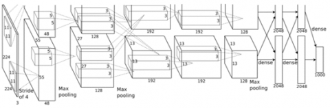
AlexNet is one of the widely used deep CNN architectures that yielded promising results in the 2012 ImageNet LSVRC-2012 Competition [38]. This architecture consists of 22 layers with Rectified Linear Unit as the activation function. AlexNet has a total of 60 million parameters, trained to identify 1000 classes. The architectural overview of AlexNet was presented in Figure 4. This architecture was modified to fit into two classes and trained from scratch with our input datasets. The input spectrograms were resized to 227 x 227 pixels and fed into the network for training. Finally, a two-way soft-max function was applied at the output layer for classification.
Figure 3. A graphical comparison between the EEG signal plots of autistic and typically developing individuals
Figure 4. Alexnet architecture as described by Krizhevsky et al. [38]
3.6 VGGNet
VGG architecture admits input images of size 224 x 224 pixels and passes them through a series of convolutional layers for feature learning and classification [39]. Rectified Linear Unit was used as the activation in all layers except the final dense layer, which was modified to fit into two classes. The input spectrograms were re-sized to 224 x 224 pixels and then fed into the network for training.
3.7 InceptionNet
The GoogLeNet was the winner of the ILSVRC 2014 and offers quite an improvement over the ZFNet (2013 winner) as well as the AlexNet (2012 winner). The concept of Inception was introduced by Szegedy et al. [40]. Subsequent versions of the GoogLeNet architecture are referred to as Inception vX, where ‘X’ refers to the number of the particular version. The GoogLeNet contains a 1x1 convolution at the middle of the network and uses a global average pooling at the end of the network instead of using the standard fully connected layers.
In an inception module, there are three convolution layers with 1x1, 3x3, and 5x5 filter sizes, along with a 3x3 max-pooling layer. These pooling and convolution layers are stacked together, where the previous layer feeds into all these layers simultaneously. The outputs from these layers are then concatenated and fed to the next module. An important feature of the inception module is the inclusion of a 1x1 bottleneck layer. The bottleneck layer exists to reduce computational costs. The entire network is 22 layers long. Inception v4 replaces the filter concatenation stage of the Inception v1 architecture with residual connections [41].
3.8 ShuffleNet
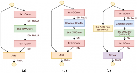
ShuffleNet was introduced as a computationally effective deep learning architecture [42]. It shuffles the input channels, such that each output channel does not relate to any of the input channels in the same group. The penultimate fully connected layer is connected to a global average pooling layer, which is then connected to a fully connected Softmax layer with two units. The pictorial overview for the ShuffleNet units is presented in Figure 5. A total of 9,37,994 parameters were trained as part of this architecture.
Figure 5. ShuffleNet units (a) bottleneck unit [43] with depthwise convolution (DWConv) [44, 45] (b) ShuffleNet unit with pointwise group convolution (GConv) and channel shuffle (c) ShuffleNet unit with stride = 2 [42]
3.9 SqueezeNet
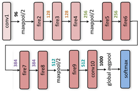
SqueezeNet is a convolutional neural network architecture developed by DeepScale, UC Berkeley, and Stanford University [46]. It scales down the neural network in terms of architecture while trying to maintain similar levels of accuracy. The 3x3 filters are substituted by 1x1 filters to reduce the number of parameters. The input channels to 3x3 filters are also decreased. Furthermore, a concept referred to as a "fire module" has been introduced in this particular architecture. A fire module has a squeeze convolutional layer (1x1 filters) which feeds into an expansion layer having both 1x1 and 3x3 convolution filters. SqueezeNet was reported to have a model size reduction of almost 50x as compared to AlexNet. The input spectrograms were fed into this architecture for classification. The pictorial overview for a SqueezeNet block is presented in Figure 6.
Figure 6. Organization of a fire module in SqueezeNet
3.10 DenseNet
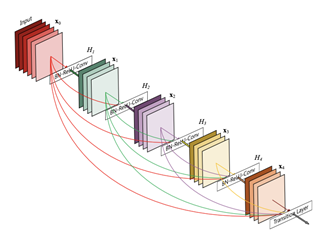
All the standard convolutional networks with ‘L’ layers have ‘L’ connections. But, DenseNet has L(L+1)/2 connections [47]. It concatenates the outputs from previous layers to subsequent layers. For each layer, the feature maps from all the preceding layers are used as inputs. This architecture is comprised of 121 layers. The model was trained with a Softmax function at its output layer. The pictorial overview of a dense block representation is presented in Figure 7.
Figure 7. A 5-layer dense block with a growth rate of k = 4. Each layer takes all preceding feature maps as input [47]
3.11 ResNet
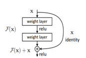
The primary feature of the ResNet architecture is the application of ‘Skip Connections’ [43]. Deep neural networks often suffer from the problem of vanishing gradients i.e. during the back-propagation phase, the gradient value decrements rapidly. This affects the convergence of the model. Skip connections are used in ResNets to address this problem. These connections will skip certain layers, which aids in minimizing the vanishing gradient problem. A pictorial overview of Skip Connections is presented in Figure 8.
Figure 8. Skip connection (or residual block) as given by He et al., 2017 [43]
The input spectrograms were re-sized to 224 x 224 pixels and then fed into the network for training. A final customized two-way Softmax layer with two units was added for classification.
To analyze the performance of the deep learning models, several experiments have been conducted on the input dataset and the observations have been discussed in this section.
4.1 Environment setup and dataset
The deep learning models were trained and run on a workstation with a Tesla K80 GPU and 12 GB of RAM. The NVidia CuDNN library was used to train the models on the GPU and accelerate the training process. The models were written in Keras library with TensorFlow as the backend. The deep neural networks were trained on the spectrograms plotted from the EEG signals with a sampling frequency of 500Hz, to classify the data into two categories: autistic or non-autistic. The classification task was binary, with the output class being ‘1’ for ASD and ‘0’ for TD. The dataset was split into two non-overlapping sets: 80% for training and 20% for testing. The test set was used for the prediction and evaluation of the deep networks.
4.2 Evaluation metrics
The performance of the deep learning models was analyzed based on metrics like Precision, Recall, and F1-score. The models which yield better results were then selected and trained again using Stratified K-Fold to further analyze and validate the results.
Precision is a measure of how precise or accurate the model is in terms of positive classifications. It measures how many examples that have been classified as positive by a network, are positive. In other words, it measures how many are “true positives” out of all the predicted positives. The relation for precision is presented in Eq. (5).
Precision $(P)=\frac{T P}{T P+F P}$ (5)
where,
TP = True Positives;
FP = False Positives.
Recall, or sensitivity is a measure of how many positives our model managed to capture out of all the predicted positive values correctly, by labeling samples as positive. The recall is calculated as presented in Eq. (6).
$\operatorname{Recall}(R)=\frac{T P}{T P+F N}$ (6)
where,
FN = False Negatives.
F1-score is a measure of the balance between the precision and recall of a model. It is calculated as presented in Eq. (7).
F1_Score $=\frac{2 * P * R}{P+R}$ (7)
Specificity is a measure of how many negatives the trained model managed to capture out of all the predicted negative values correctly, by labeling samples as negative. The relation for calculating specificity is presented in Eq. (8).
Specificity $(S)=\frac{T N}{T N+F P}$ (8)
where,
TN = True Negatives.
4.3 Performance analysis
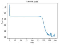
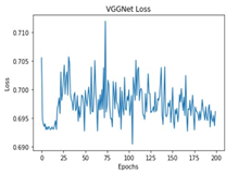
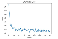
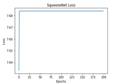
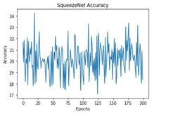
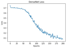
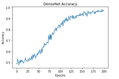
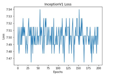
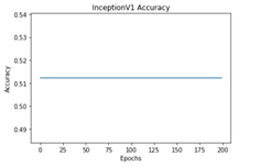
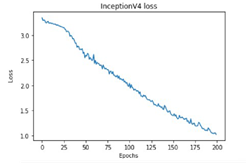
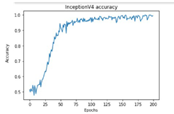
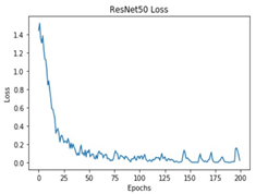
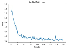
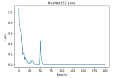
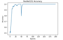
The performance of the training process for different deep learning models was analyzed based on Accuracy and Loss.
All these models were trained for 200 epochs and the resultant observations have been presented below (Table 1).
Table 1. Observations of the training process for different deep learning models
|
S.No |
Model |
Loss |
Accuracy |
|
1. |
AlexNet |
||
|
2. |
VGGNet |
||
|
3. |
ShuffleNet |
||
|
4. |
SqueezeNet |
||
|
5. |
DenseNet |
||
|
6. |
InceptionV1 |
||
|
7. |
InceptionV4 |
||
|
8. |
ResNet50 |
||
|
9. |
ResNet101 |
||
|
10. |
ResNet152 |
Table 2. Analysis of performance measures for different deep learning models
|
Model |
Training Accuracy (in %) |
Testing Accuracy(in %) |
Precision |
Recall (Sensitivity) |
F1-Score |
Specificity |
|
AlexNet |
52.45 |
50.98 |
0.43 |
0.43 |
0.45 |
0.45 |
|
VGGNet |
50.37 |
51.96 |
0.25 |
0.50 |
0.33 |
0.00 |
|
ShuffleNet |
94.28 |
44.12 |
0.43 |
0.44 |
0.39 |
0.16 |
|
SqueezeNet |
52.33 |
49.02 |
0.25 |
0.50 |
0.33 |
0.00 |
|
DenseNet |
96.67 |
48.53 |
0.21 |
0.22 |
0.21 |
0.29 |
|
InceptionV1 |
50.98 |
60.98 |
0.26 |
0.51 |
0.35 |
0.00 |
|
InceptionV4 |
91.34 |
53.92 |
0.55 |
0.54 |
0.55 |
0.55 |
|
ResNet50 |
92.52 |
81.91 |
0.92 |
0.91 |
0.91 |
1.00 |
|
ResNet101 |
96.08 |
47.55 |
0.53 |
0.51 |
0.51 |
0.55 |
|
ResNet152 |
91.30 |
51.96 |
0.44 |
0.44 |
0.44 |
0.37 |
Table 3. Results of K-fold cross validation across 5 folds for variants of ResNet and DenseNet architectures
|
Model |
Accuracy in Percentage |
|||||
|
Fold-1 |
Fold-2 |
Fold-3 |
Fold-4 |
Fold-5 |
Average |
|
|
ResNet50 |
49.02 |
73.04 |
93.63 |
97.06 |
96.77 |
81.91 |
|
ResNet101 |
47.31 |
46.24 |
59.14 |
49.16 |
49.46 |
50.66 |
|
ResNet152 |
51.46 |
56.86 |
37.25 |
51.96 |
55.88 |
50.68 |
|
DenseNet |
48.53 |
49.02 |
45.59 |
52.94 |
50.98 |
49.41 |
From Table 2, it can be observed that although the training performance of AlexNet, VGGNet, ShuffleNet and SqueezeNet were considerable, it did not perform well for testing sets. It is to be noted that the ResNet and DenseNet architectures yielded considerably better performances for training, and testing sets. Hence, the next step involves the application of stratified K-fold cross-validation to analyze the performance of these networks.
The observations obtained for the 5-fold cross-validation process ResNet50, ResNet101, ResNet152 and DenseNet are reported in Table 3. From Table 3, it could be observed that ResNet50 based deep architecture was able to detect ASD from EEG signals with an average accuracy of 81%. Hence, it was concluded that ResNet50 based deep architecture can be employed for ASD detection from input spectrograms. The Skip Connections between layers in the ResNet architecture add the outputs from previous layers to the outputs of stacked layers. This results in the ability to train much deeper networks than what was previously possible in the other networks. The feature concatenation between multiple layers enabled the network to identify distinctive features in the input spectrogram pattern and thereby exhibiting high performance. Having observed this performance improvement, this architecture can be adapted for other biomedical signals towards effective disease detection.
This research extends the scope of objective assessment methods closer towards non-clinical experts for the effective diagnosis of ASD using deep learning techniques. The key objective of this work is to examine the performances of state-of-the-art deep convolutional networks for the detection of ASD from EEG signals. Extensive analysis was performed with different deep architectures like AlexNet, VGGNet, ShuffleNet, SqueezeNet, DenseNet, InceptionNet, and ResNet. To the best of our knowledge, this is the first work that presents the quantitative analysis of the above-mentioned deep architectures for ASD detection. The performances of these methods were analyzed with metrics like specificity, sensitivity, and F1-score. Observations from different experiments revealed that the ResNet50 based deep convolutional network performs better than the other architectures in detecting ASD, with an average accuracy of 81.91 %. The future scope of this research involves layer-wise fine-tuning of the ResNet50 architecture with larger datasets to further improve the accuracy.
This research was funded by the Department of Science and Technology DST under Science for Equity, Empowerment, and Development (SEED) Division (File No: SEED/TIDE/092/2016). We would like to render our sincere thanks to the Sri Ramachandra Institute of Higher Education and Research for their kind support and assistance in data acquisition.
[1] Park, H.R., Lee, J.M., Moon, H.E., Lee, D.S., Kim, B.N., Kim, J., Paek, S.H. (2016). A short review on the current understanding of autism spectrum disorders. Experimental Neurobiology, 25(1): 1-13. https://doi.org/10.5607/en.2016.25.1.1
[2] Baio, J., Wiggins, L., Christensen, D.L., Maenner, M.J., Daniels, J., Warren, Z., Dowling, N.F. (2018). Prevalence of autism spectrum disorder among children aged 8 years—autism and developmental disabilities monitoring network, 11 sites, United States, 2014. MMWR Surveillance Summaries, 67(6): 1-11. https://doi.org/10.15585/mmwr.ss6706a1
[3] Spain, D., Sin, J., Linder, K.B., McMahon, J., Happé, F. (2018). Social anxiety in autism spectrum disorder: A systematic review. Research in Autism Spectrum Disorders, 52: 51-68. https://doi.org/10.1016/j.rasd.2018.04.007
[4] American Psychiatric Association. (2013). Diagnostic and Statistical Manual of Mental Disorders, Text.
[5] Thabtah, F., Peebles, D. (2019). Early autism screening: A comprehensive review. International Journal of Environmental Research and Public Health, 16(18): 3502. https://doi.org/10.3390/ijerph16183502
[6] Olejniczak, P. (2006). Neurophysiologic basis of EEG. Journal of Clinical Neurophysiology, 23(3): 186-189. https://doi.org/10.1097/01.wnp.0000220079.61973.6c
[7] Lindsley, D.B. (1936). Brain potentials in children and adults. Science, 84(2181): 354. https://doi.org/10.1126/science.84.2181.354
[8] Grastyan, E., Lissak, K., Madarasz, I., Donhoffer, H. (1959). Hippocampal electrical activity during the development of conditioned reflexes. Electroencephalography and Clinical Neurophysiology, 11(3): 409-430. https://doi.org/10.1016/0013-4694(59)90040-9
[9] Welsh, J.P., Estes, A.M. (2018). Autism: Exploring the social brain. eLife, 7: e35392. https://doi.org/10.7554/eLife.35392
[10] Dover, C.J., Le Couteur, A. (2007). How to diagnose autism. Archives of Disease in Childhood, 92(6): 540-545. http://dx.doi.org/10.1136/adc.2005.086280
[11] Russell, S.J., Norvig, P. (2016). Artificial intelligence: A modern approach. Malaysia; Pearson Education Limited.
[12] Cortes, C., Vapnik, V. (1995). Support-vector networks. Machine Learning, 20(3): 273-297. https://doi.org/10.1007/BF00994018
[13] Breiman, L. (2017). Classification and regression trees. Routledge.
[14] Breiman, L. (2001). Random forests. Machine Learning, 45(1): 5-32. https://doi.org/10.1023/A:1010933404324
[15] Parikh, M.N., Li, H., He, L. (2019). Enhancing diagnosis of autism with optimized machine learning models and personal characteristic data. Frontiers in Computational Neuroscience, 13: 1-9. https://doi.org/10.3389/fncom.2019.00009
[16] Grether, J.K., Anderson, M.C., Croen, L.A., Smith, D., Windham, G.C. (2009). Risk of autism and increasing maternal and paternal age in a large North American population. American Journal of Epidemiology, 170(9): 1118-1126. https://doi.org/10.1093/aje/kwp247
[17] Plitt, M., Barnes, K.A., Martin, A. (2015). Functional connectivity classification of autism identifies highly predictive brain features but falls short of biomarker standards. NeuroImage: Clinical, 7: 359-366. https://doi.org/10.1016/j.nicl.2014.12.013
[18] Duda, M., Ma, R., Haber, N., Wall, D.P. (2016). Use of machine learning for behavioral distinction of autism and ADHD. Translational Psychiatry, 6(2): 1-32. https://doi.org/10.1038/tp.2015.221
[19] Chen, C.P., Keown, C.L., Jahedi, A., Nair, A., Pflieger, M.E., Bailey, B.A., (2015). Diagnostic classification of intrinsic functional connectivity highlights somatosensory, default mode, and visual regions in autism. NeuroImage: Clinical, 8: 238-245. https://doi.org/10.1016/j.nicl.2015.04.002
[20] Boutros, N.N., Lajiness-O’Neill, R., Zillgitt, A., Richard, A.E. Bowyer, S.M. (2015). EEG changes associated with autistic spectrum disorders. Neuropsychiatric Electrophysiology, 1(1): 1-3. https://doi.org/10.1186/s40810-014-0001-5
[21] Sheikhani, A., Behnam, H., Mohammadi, M.R., Noroozian, M., Mohammadi, M. (2012). Detection of abnormalities for diagnosing of children with autism disorders using of quantitative electroencephalography analysis. Journal of Medical Systems, 36(2): 957-963. https://doi.org/10.1007/s10916-010-9560-6
[22] Choe, S.H., Chung, Y.G., Kim, S.P. (2010). Statistical spectral feature extraction for classification of epileptic EEG signals. In 2010 International Conference on Machine Learning and Cybernetics, 6: 3180-3185. https://doi.org/10.1109/ICMLC.2010.5580709
[23] Bascil, M.S., Tesneli, A.Y., Temurtas, F. (2016). Spectral feature extraction of EEG signals and pattern recognition during mental tasks of 2-D cursor movements for BCI using SVM and ANN. Australasian Physical & Engineering Sciences in Medicine, 39(3): 665-676. https://doi.org/10.1007/s13246-016-0462-x
[24] Tsipouras, M.G. (2019). Spectral information of EEG signals with respect to epilepsy classification. EURASIP Journal on Advances in Signal Processing, 2019(1): 1-10. https://doi.org/10.1186/s13634-019-0606-8
[25] Acharya, U.R., Sree, S.V., Chattopadhyay, S., Yu, W., Ang, P.C.A. (2011). Application of recurrence quantification analysis for the automated identification of epileptic EEG signals. International Journal of Neural Systems, 21(3): 199-211. https://doi.org/10.1142/S0129065711002808
[26] Heunis, T., Aldrich, C., Peters, J.M., Jeste, S.S., Sahin, M., Scheffer, C., De Vries, P.J. (2018). Recurrence quantification analysis of resting state EEG signals in autism spectrum disorder–A systematic methodological exploration of technical and demographic confounders in the search for biomarkers. BMC Medicine, 16(1): 1-17. https://doi.org/10.1186/s12916-018-1086-7
[27] Bosl, W.J., Loddenkemper, T., Nelson, C.A. (2017). Nonlinear EEG biomarker profiles for autism and absence epilepsy. Neuropsychiatric Electrophysiology, 3(1): 1-13. https://doi.org/10.1186/s40810-017-0023-x
[28] Deng, L., Yu, D. (2014). Deep learning: methods and applications. Foundations and Trends® in Signal Processing, 7(3-4): 197-387. https://doi.org/10.1561/2000000039
[29] Tabar, Y.R., Halici, U. (2016). A novel deep learning approach for classification of EEG motor imagery signals. Journal of Neural Engineering, 14(1): 16-30. https://doi.org/10.1088/1741-2560/14/1/016003
[30] Vincent, P., Larochelle, H., Lajoie, I., Bengio, Y., Manzagol, P.A. (2010). Stacked denoising autoencoders: Learning useful representations in a deep network with a local denoising criterion. Journal of Machine Learning Research, 11: 3371-3408.
[31] Yıldırım, Ö., Baloglu, U.B., Acharya, U.R. (2018). A deep convolutional neural network model for automated identification of abnormal EEG signals. Neural Computing and Applications, 32: 15857-15868. https://doi.org/10.1007/s00521-018-3889-z
[32] Zabihi, M., Rad, A.B., Kiranyaz, S., Särkkä, S., Gabbouj, M. (2019). 1d convolutional neural network models for sleep arousal detection. arXiv preprint arXiv:1903.01552.
[33] Wu, Y., Yang, F., Liu, Y., Zha, X., Yuan, S. (2018). A comparison of 1-D and 2-D deep convolutional neural networks in ECG classification. IEEE Engineering in Medicine and Biology Society.
[34] Liu, Q., Cai, J., Fan, S.Z., Abbod, M.F., Shieh, J.S., Kung, Y., Lin, L. (2019). Spectrum analysis of EEG signals using CNN to model patient’s consciousness level based on anesthesiologists’ experience. IEEE Access, 7: 53731-53742. https://doi.org/10.1109/ACCESS.2019.2912273
[35] Kwon, Y.H., Shin, S.B., Kim, S.D. (2018). Electroencephalography based fusion two-dimensional (2D)-convolution neural networks (CNN) model for emotion recognition system. Sensors, 18(5): 1383. https://doi.org/10.3390/s18051383
[36] Ozdemir, M.A., Degirmenci, M., Guren, O., Akan, A. (2019). EEG based emotional state estimation using 2-D deep learning technique. In 2019 Medical Technologies Congress (TIPTEKNO), pp. 1-4. https://doi.org/10.1109/TIPTEKNO.2019.8895158
[37] World Medical Association. (2001). World medical association declaration of Helsinki. ethical principles for medical research involving human subjects. Bulletin of the World Health Organization, 79(4): 373-374.
[38] Krizhevsky, A., Sutskever, I., Hinton, G.E. (2012). Imagenet classification with deep convolutional neural networks. In Advances in Neural Information Processing Systems, 1097-1105.
[39] Simonyan, K., Zisserman, A. (2015). Very deep convolutional networks for large-scale image recognition. Published as a Conference Paper at ICLR 2015.
[40] Szegedy, C., Liu, W., Jia, Y., Sermanet, P., Reed, S., Anguelov, D., Erhan, D., Vanhoucke, V. Rabinovich, A. (2015). Going deeper with convolutions. In Proceedings of the IEEE Conference on Computer Vision and Pattern Recognition, pp. 1-9.
[41] Szegedy, C., Ioffe, S., Vanhoucke, V., Alemi, A.A. (2017). Inception-v4, inception-Resnet and the impact of residual connections on learning. In Thirty-First AAAI Conference on Artificial Intelligence, 31(1). Retrieved from https://ojs.aaai.org/index.php/AAAI/article/view/11231.
[42] Zhang, X., Zhou, X., Lin, M., Sun, J. (2018). Shufflenet: An extremely efficient convolutional neural network for mobile devices. In Proceedings of the IEEE Conference on Computer Vision and Pattern Recognition, pp. 6848-6856.
[43] He, K., Zhang, X., Ren, S., Sun, J. (2016). Deep residual learning for image recognition. 2016 IEEE Conference on Computer Vision and Pattern Recognition (CVPR), pp. 770-778. https://doi.org/10.1109/CVPR.2016.90
[44] Chollet, F. (2017). Xception: Deep learning with depthwise separable convolutions. In Proceedings of the IEEE Conference on Computer Vision and Pattern Recognition, pp. 1251-1258.
[45] Howard, A.G., Zhu, M., Chen, B., Kalenichenko, D., Wang, W., Weyand, T., Adam, H. (2017). Mobilenets: Efficient convolutional neural networks for mobile vision applications. arXiv preprint arXiv:1704.04861.
[46] Iandola, F.N., Han, S., Moskewicz, M.W., Ashraf, K., Dally, W.J., Keutzer, K. (2016). SqueezeNet: AlexNet-level accuracy with 50x fewer parameters and < 0.5 MB model size. arXiv preprint arXiv:1602.07360.
[47] Huang, G., Liu, Z., Van Der Maaten, L., Weinberger, K.Q. (2017). Densely connected convolutional networks. 2017 IEEE Conference on Computer Vision and Pattern Recognition (CVPR), pp. 2261-2269. https://doi.org/10.1109/CVPR.2017.243