Sema Yildirim* | Hasan Erdinc Kocer | Ahmet Hakan Ekmekci
© 2021 IIETA. This article is published by IIETA and is licensed under the CC BY 4.0 license (http://creativecommons.org/licenses/by/4.0/).
OPEN ACCESS
Persistent, unchanging, and non-reactive focal or generalized abnormal Slow Wave (SW) activities in an awake adult patient are examined pathologically. Although these waves in Electroencephalogram (EEG) are much less prominent than transient activities in some areas, it is not possible to understand them easily by looking at the EEG. For this reason, reliable computer programs that can sort out Slow Waves (SWs) correctly are needed. In this study, a new method based on MinPeakProminence that can detect abnormal SW activities was developed. To test the performance of the study, the data collected from Selcuk University Hospital (22 subjects - epilepsy and various neurological diseases) and Bonn Hospital (only normal A dataset) were used. Various statistical performance measurement methods were used to search the results. The results of this analysis revealed that the classification success, sensitivity and specificity values obtained with the SUH dataset were 96.5%, 93.3% and 96.1%, respectively. In the results of the experiments made with the Bonn dataset, 100% classification success was achieved. Besides, according to the analyses, it was found that SWs are frequently seen in the posterior regions of the brain, especially in the parietal and occipital regions in the SUH dataset.
electroencephalogram, slow wave, peak, minpeakprominence, epilepsy, neurologic disorder
Electroencephalography (EEG) is a technique where the electrical activities of the brain are recorded and it has an important place in the diagnosis of neurological diseases. With the developments in signal processing studies in recent years, it is possible to reveal the hidden and important signals in EEG. For example, changes in amplitude and frequency in background activities may indicate a lesion. In addition, epileptiform activities determined in the EEG signal also contribute greatly to the diagnosis of epilepsy [1].
Epilepsy is a chronic neurological disease that occurs as a result of abnormal and excessive electrical discharge in cortical neurons and the essential syndrome which is characterized by recurrent epileptic seizures [2].
In the most common definition made by the International League Against Epilepsy (ILAE), epilepsy is a transient functional disorder of the central nervous system caused by excessive and synchronous abnormal neuronal activity in the cortex [3-7]. This neurological disease, which occurs as a consequence of recurrent seizures, negatively influences around 1% of the world population [8]. Even with the use of various medications and surgical treatment, seizures cannot be controlled in more than 25% of epilepsy patients. Due to the incapability to detect the occurrence of seizures in advance, sudden and unexpected deaths occur in some patients with this disease or the risk of morbidity increases [9].
The World Health Organization (WHO) reports that about 50 million people worldwide have epileptic seizures, according to epidemiological data. It was revealed in a recent study that epilepsy is one of the severest disorders among neurological diseases [10].
It is known that epilepsy is the most common in childhood and adolescence, and the second most common after cerebrovascular diseases in adults. In spite of its widespread prevalence, various difficulties are encountered in establishing the definitive diagnosis of epilepsy, especially in distinguishing it from psychogenic seizures. To eliminate these difficulties and to obtain more precise and clear results, Video-EEG imaging (VEEG) method is used. However, this imaging technique, a gold standard in the differentiation of non-epileptic seizures and epilepsy, has a limited use because of the difficulties faced in its application and its high cost. Due to these reasons, this technique is often preferred to be used in situations where a decision cannot be made with anamnesis, clinical examination, and EEG [11].
Before starting EEG, an EEG procedure suitable for the patient should be selected, taking into account their clinical information. The recorded signals should be carefully examined and interpreted because spikes or other recorded abnormalities that have been observed contain useful information in diagnosis and treatment [12]. Despite the advances in technology, the EEG recordings are mostly interpreted manually. Manual review/examination of EEG recordings of 20-30 minutes or even hours takes quite a long time [13, 14]. To make a faster and more accurate diagnosis, various signal processing algorithms and computer programs have been developed in recent years [15]. In studies regarding automated EEG analysis, seizures, spikes, and sharp waves, mostly indicative of epileptic activity, were examined [13, 14]. Focal slow waves in the delta and theta frequency range are often evaluated as psychopathological. Therefore, such waves with high amplitude and low frequency activity are very important in the electroencephalogram. Wienbruch et al. aimed to detect focal slow wave activities. In their study, they compared the records of the patients diagnosed with schizophrenia and affective disorder with normal records [16]. In another study, a method was developed for detecting Slow Wave Sleep (SWS) on an automatic single channel in sleep EEG. With this study, the uncertainty caused by individual differences was minimized, and the effects of the SWS ratio on the effectiveness of sleep staging were investigated [17]. On the other hand, there has not been sufficient number of studies on the analysis of slow-waves since they vary more greatly than the morphology of sharp transients [18]. However, Slow Waves (SWs) are as important as spikes in both clinical diagnosis and automatic detection [19]. For this reason, in this study, a new MinPeakProminence-based (MPP) method has been developed for the detection of Slow Wave (SW), which is an indicative of EEG anomaly. The aim of this method is to determine the relationship of SW activities with epilepsy and other neurological diseases and to detect which regions of the brain are frequently seen (focal, lateralized, and generalized). Consequently, in this study, a new MPP-based method has been generated for the detection of SWs, which is the sign of EEG anomaly. With this method, it is intended to find out the relevance of SW activities with epilepsy and other neurological diseases and to locate which regions of the brain are commonly seen (focal, lateralized, generalized).
The other parts of this paper are organized as follows. In Section II, the methods that form the basis of the whole study and the datasets used are mentioned. The experimental results obtained with the performed method are discussed in Section III. Finally, Section IV presents a brief summary of the study and the scope of future research.
2.1 Electroencephalography (EEG)
Figure 1. EEG electrode placements and polarity scheme. The signal sample taken from the electrode pairs formed by bipolar EEG recording of a subject in the Selcuk University Hospital (SUH) dataset is shown (Scale 50 on EEGLab)
The method of recording brain waves from the human scalp is called EEG. The interpretation of the signals obtained by this method is quite significant for diagnosis [20]. Especially the conditions that cause epileptic disorders are accurately determined with the correct analysis of EEG signals (EEGs) [8]. Since EEG, which is used especially in the diagnosis of epilepsy, is a non-invasive and inexpensive method, it is currently used as the most frequently used method in diagnosis and treatment guidance. The diagnosis is made mainly by detecting marked asymmetry or slowing of the ground activity and epileptiform discharges (spike, sharp and spike-wave discharges) in the patient whose EEG record has been taken. Moreover, many epileptic patients can constantly show normal EEG findings in the interictal period. As it is hard to detect seizures with low frequency in ictal period with EEG recording, it is often not helpful in diagnosis in such cases. However, EEG is quite beneficial for the evaluation of focal or dynamic cerebral function thanks to its precise temporal sensitivity [21-24].
Vertical areas show stresses and horizontal areas show the time in a standard EEG. In this way, an almost real-time image of cerebral activity is obtained (Figure 1).
2.2 EEG placement/montages
Selecting the proper EEG montage is quite significant for diagnosis as it reveals rhythm indicative of anomalies [25].
There are two types of EEG recordings, depending on the way the signal is received from the head (from the scalp or intracranial). Electrodes that provide electrical contact in the type of recording taken from the scalp are placed on the scalp. In intracranial EEG, private electrodes are implanted in the brain by surgical operation.
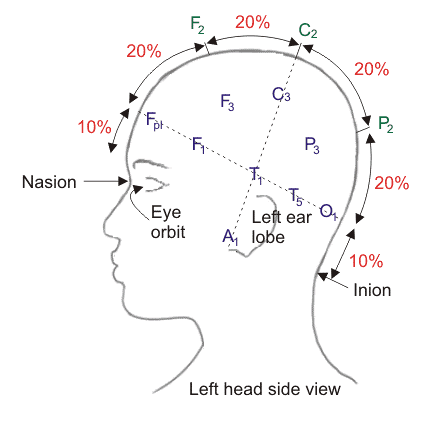
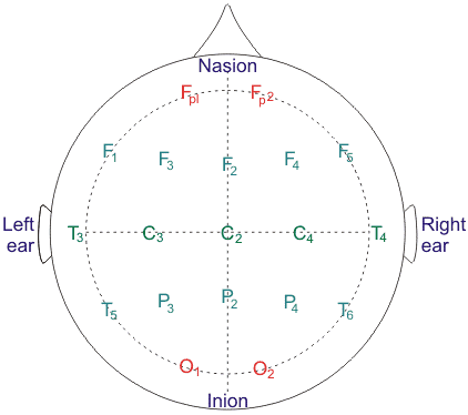
Electrodes are adjoined to the scalp according to the International 10/20 Electrode placement system in a standard EEG recording taken from the scalp. This placement system is essentially based on the distances between the marks indicating bony parts on the head. Then, the electrodes are placed at intervals between 10 and 20 percent of the total length of these lines. Each electrode position is identified by a letter and a given number. The letters (Fp, frontopolar; F, frontal; C, central; T, temporal; P, parietal; O, occipital, lower case "z", midline position of the scalp) indicate the position of the electrode on the head, and the numbers (electrodes in the left hemisphere are indicated by odd numbers, and electrodes in the right hemisphere as even numbers) indicate the brain hemisphere (Figure 2). This method enables the signals received from the same parts of the patients with different head sizes to be recorded in a standard way. On the other hand, the 10/20 system can be divided into smaller proportional distances to ensure a more precise recording of electrical activity.
(a)
(b)
Figure 2. International 10/20 electrode placements in a bipolar montage (a) Side view (b) Top view [26]
After making the necessary calibration settings and determining the correct display of EEG recording, the EEG montage should be continued. Although there are many different types of montages used for EEG, they are roughly divided into two groups: monopolar and bipolar recording. In monopolar montages, each electrode is connected to a single reference point. This reference can be another electrode on the scalp or a mathematical combination of signals like a mathematical average reference. The bipolar montages consist of electrode chains connected to one or two adjacent electrodes. Another type of montage used for the evaluation of epilepsy is the Laplacian or source derivation montage in which each active recording electrode is compared to the mathematical weighted average of the surrounding electrodes. With the combined use of these montage techniques stated above, all abnormalities in EEG are rather beneficial not only as a reflection of the signal imaging method, but also for determining pathological conditions [27].
2.3 EEG frequency bands and waveforms
Another vital issue to be considered in EEG recording is waveforms and frequency bandwidths. These waveforms and predominant frequencies (e.g., alert wakefulness, drowsiness, sleep), varying from patient to patient, are of great importance as they contain findings for the detection of the disease.
Characteristics such as frequency/wavelength, voltage/amplitude, and waveform, eye blinking reactivity, hyperventilation and photic stimulation should be considered in the visual examination of EEG recordings. It is also necessary to define the spatial range (local or generalized, unilateral or bilateral) and temporal persistence (sporadic and short or long and persistent) of abnormalities [8].
Changes in EEG rhythms are associated with transient activities such as spike waves, multiple spikes and sharp waves. However, the main point here is the changes in the amplitude and frequency of the EEG rhythms [28]. Recent researches have shown that more accurate information can be obtained from EEG basic rhythms about neuronal activities such as various brain functioning and pathology states [10, 29]. Therefore, a detailed description of the waveforms and frequency bandwidths of the basic EEG waves is given in Table 1 [30-32].
Even though EEG includes a wide variety of frequency components, the range of clinical and physiological concern is between 0.3 and 30 Hz.
The typical frequency ranges of sudden waves, sharp waves and SWs that are especially associated with cognitive processes in decision making and attention processes are 13.5–50 Hz, 5–12.5 Hz, and 0.5–4 Hz, respectively [33-36].
2.4 Slow wave activity
The most critical anomalies considered in epilepsy are spike waves, sharp waves, and short transient waves called spike wave complexes. These waveforms can take place in recurrent (polyspike and spike-wave) patterns [37]. Ictal or interictal EEG recordings of almost all epilepsy patients indicate similar characteristics. These similar characteristics in EEG recordings include many waveforms spikes, sharp waves, spike and waves, multiple spikes, multiple spike and waves, periodic sharp waves, slow wave complexes, and paroxysmal fast activity [38-45]. The most crucial thing to do before interpreting such activities is to pay attention to the background. A correct interpretation of the frequency, amplitude, and degree of synchronization can enable sufficient information about the background EEG.
Slow theta or delta waves can be observed in an awake person, albeit temporarily. This condition generally occurs with the drowsiness of the person. Whereas these generalized activities are considered normal in children, adolescents, young adults, and some elderly individuals, the intermittent or diffuse, focal or general, theta or delta frequency observed in the EEG of an awake adult and the intermittent slowing of the background indicate pathology (Figure 3). In other words, background slowing may indicate diffuse or focal cerebral dysfunction.
Background slowing is basically divided into two groups: focal slowing and general slowing. Focal slowing is an indication of focal cerebral pathology of the brain area. The slowing can be intermittent or permanent. Intermittent focal slowing may occur depending on the effects of a sedative or hypnotic drug. Examples of intermittent focal slowing may include stroke, cerebral hemorrhage, tumors, traumatic injury, malformations of cortical development, focal epileptic focus, arteriovenous malformations, and temporary or permanent ischemia resulting from focal brain infection [15]. General background slowing resembles focal slowing, but it indicates diffuse cerebral dysfunction. The effects of sedative centrally acting medications, neurodegenerative disorders, hydrocephalus, metabolic or toxic encephalopathy, central nervous system (CNS) infectious disorders, and focal midline structural lesions such as meningoencephalitis may cause general background slowing. Other epileptiform EEG abnormalities that could provide clues about the abnormal area are focal or lateralized slowing or activity asymmetry in both hemispheres [46].
Table 1. Main characteristics features of the brain waves
|
Frequency band |
Frequency |
Brain states |
|
Gamma (γ) |
>32 Hz |
Gamma waves have a fairly high frequency band and are frequently filtered in EEG recordings due to the lack of clinical and physiological interest. |
|
Beta (β) |
12-35 Hz |
Beta waves are mostly observed in the frontal areas. They are increased with expectancy states and tension. |
|
Alpha (α) |
8-12 Hz |
Alpha waves are seen in normal adults in awake states in which they are not relaxed and mentally active. Although the amplitude is often less than 50 µV, they are often prominent in the occipital areas. |
|
Theta (θ) |
4-8 Hz |
Theta waves are seen in normal situations in babies and children, and in adults during drowsiness and sleep. This waveform is rarely seen in normal and awake adults. The high theta activity in awake adults point out abnormal and pathological conditions as in delta waves. |
|
Delta (δ) |
0.5-4 Hz |
Delta waves are predominantly observed during the deep sleep stages of normal adults. Other situations indicate pathology [28]. |
Figure 3. Background slowing (Longitudinal bipolar montage). Routine EEGs of a 38-years-old subject with epilepsy included in the SUH dataset. a) Background theta and delta slowing in many channels in seconds 120-123, b) in seconds 126-129, and c) theta and delta slowing observed in almost all channels in seconds 133-135. These findings are abnormal for the EEG recorded while awake, and indicate an abnormality as noted in the subject's clinical history
Table 2. The lowest and highest value ranges used in the detection of peaks [47]
|
Peak Number |
Left Interval Lies Between Peak and |
Right Interval Lies Between Peak and |
Lowest Point on the Left Interval |
Lowest Point on the Right Interval |
Reference Level (Highest Minimum) |
|
1 |
Left end |
Crossing due to peak 2 |
Left endpoint |
a |
a |
|
2 |
Left end |
Right end |
Left endpoint |
h |
Left endpoint |
|
3 |
Crossing due to peak 2 |
Crossing due to peak 4 |
b |
c |
c |
|
4 |
Crossing due to peak 2 |
Crossing due to peak 6 |
b |
d |
b |
|
5 |
Crossing due to peak 4 |
Crossing due to peak 6 |
d |
e |
e |
|
6 |
Crossing due to peak 2 |
Right end |
d |
h |
d |
|
7 |
Crossing due to peak 6 |
Crossing due to peak 8 |
f |
g |
g |
|
8 |
Crossing due to peak 6 |
Right end |
f |
h |
f |
|
9 |
Crossing due to peak 8 |
Crossing due to right endpoint |
h |
i |
i |
2.5 Minpeakprominence Method (MPP)
As mentioned in the previous sections, EEGs are generally divided into four frequency bands, and the focus of this study has been on delta and theta waves. For the detection of these waves, generally called SWs, a method based on MPP has been developed.
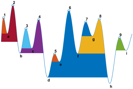
Figure 4. Detection of the peaks of a signal with MPP
MPP is a method used to detect only peaks of least relative importance of a given value. This method is used to detect more prominent peaks as opposed to selection by absolute value. The MPP method compares each neighbouring peak with each other and detects only the peaks that are most important to the specified level. The steps followed to detect the significant peaks of a signal shown in Figure 4 are detailed in Table 2.
Examining the peaks of the signal in the example, it was observed that the signal passed the last value on the left for the left interval value and peak 2 for the right interval value. Consequently, the highest minimum peak for peak number 1 was determined as a. As explicitly presented in the table, each peak is detected individually in compliance with the minimum interior height and the location of the other peaks, through this method.
The following steps are operated when measuring the prominence of any peak:
A marker is placed at the peak.
Then, a horizontal line from above peak to left and right is extended until one of the following operations is performed.
If there is a higher peak it will pass this signal.
If not, the line is delivered to the left or right end of the signal.
The minimum value of the signal is calculated in each of the two intervals defined in step 2. This point is either a valley or one of the signal endpoints.
The peak stands out when these two intervals are higher than the minimum value.
Figure 5 shows a graph that enables the determination of important peaks of a signal with MPP. In this example, peaks with a significance of at least 4 were detected. Here, according to the aforementioned process steps, a marker is first placed on a peak, then higher peaks are searched. Significant peaks are detected when the peak marked last is higher than the minimum value of the two intervals.
Figure 5. Graph showing the significant peaks of a signal (for MPP=4) [48]
2.6 Data collection
EEGs and clinical information of 22 subjects (the average age of 12 males’ patients is 43, and the average age of 10 females’ patients is 49) who were diagnosed with epilepsy and other neurological disorders and who came to the SUH dataset due to various complaints (Non-Invasive Clinical Research Ethics Committee No. 2014/423) were collected retrospectively (in April and December, 2014).
The distribution chart of the ages of these patients, whose average age range value is specified, is shown in Figure 6 in detail. When the Figure 6 was examined, it was observed that patients diagnosed with neurological disorders were especially between the ages of 40-60. EEGs of the subjects were obtained through bipolar montage using the 10/20 system EEG placement. During the routine EEG recording, 20 electrodes were connected, and the information of the last two channels (19th channel Electrocardiography (ECG), 20th channel Photic Stimulation) was not processed since it did not contain any information to describe neurological disorders. That’s why the focus was on the signals obtained with 18 electrodes.
Signal amplitude value is 150 µVp-p from peak to peak, and sampling frequency is 200. Also, 1.0 and 15.0 were applied for the low-pass Notch filter and the high-pass Notch filter, respectively.
The study did not include personal data of the subjects. The clinical information and inclusion criteria obtained as a consequence of the visual examination of these subjects are presented in Table 3. EEG records of subjects younger than 18 years old and older than 70 years were excluded in the data in the study, in accordance with the opinions and recommendations of the attending physician.
Some statistical characteristics of the same subjects in the dataset are introduced in Table 4. It is clearly seen in this table that the mean age of male and female subjects included in the dataset is 45.27. Some of these subjects in the dataset received drug treatment (14 subjects receiving medication) and some (8 subjects not receiving medication) did not. However, this information was not recorded in the clinical reports of the subject who did not receive medication either because the subject was newly diagnosed or due to inadequate clinical information (EEG laborant forgetting to ask, subject not remembering, etc.). Besides, subject records with missing such clinical information were eliminated from the study. 15 of these people coming to the hospital with various complaints were diagnosed with epilepsy, and 7 were diagnosed with different neurological diseases (encephalitis, shivering pain, etc.). Moreover, all other statistical features such as the distribution of diseases by gender and the ratio of the number of subjects to each other are also presented in detail in this Table 4.
Although EEG records performed over 30 minutes are crucial for diagnosis and treatment, this duration is kept very short because of insufficient cost and limited time. Therefore, EEG records are generally performed for an average of 20 to 30 minutes. Recording durations differ from each other. Therefore, the sizes of the EEG records of each subject are different depending on these durations. EEG page numbers (every page includes 15-sec x 200 sample rates) and file sizes in the SUH dataset are given in Table 5. When the file sizes in the table are examined, the shortest and longest EEG file sizes are 144000 and 192000, respectively.
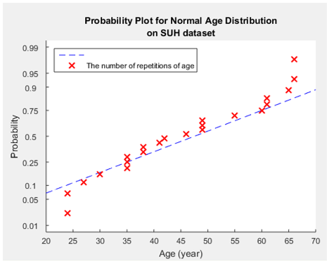
Figure 6. Graph of the probability plot for normal age distribution on SUH dataset
The repetition numbers of the EEG page numbers are presented in Table 6, and the frequencies of the page numbers are shown in Figure 7 as the probability distribution for a better analysis. As it is seen in Figure 7, the number of pages of EEG records recorded in the highest number is between 57 and 60. In other respects, the least frequent pages are 48, 53, 56, and 64. Consequently, it can be simply said that routine EEG records for this dataset include an average of 58.5 (for 57, 58, 59 and 60) pages. The average duration of the recordings (58.5 / 4≈15 minutes) is 15 minutes. As mentioned in the previous sections, routine EEG recording durations are actually around 20-30 minutes. EEG recordings taken during these durations often contain artefacts. These artefacts can hinder algorithmic analysis and visual inspection. It was observed in this dataset that some parts of the recordings were either empty or entirely filled with artefacts because of some reasons such as the movement of most subjects and loose contact caused by the disconnection of the electrode connections. For this reason, such recordings that do not form connections were eliminated from the EEG recordings.
Table 3. Personal information and clinical characteristics of the subjects included in the SUH dataset
|
Subject (gender, age) |
Diagnosis |
Drug (Yes/No) |
|
suh-01 (M 38) |
Epilepsy |
Yes |
|
suh-02 (M 24) |
Epilepsy |
Yes |
|
suh-03 (F 42) |
Epilepsy |
No |
|
suh-04 (M 60) |
Psychogenic seizure |
No |
|
suh-05 (F 38) |
Epilepsy |
No |
|
suh-06 (F 27) |
Epilepsy |
Yes |
|
suh-07 (M 24) |
Encephalitis |
Yes |
|
suh-08 (M 35) |
Cerebrovascular |
Yes |
|
suh-09 (M 46) |
Epilepsy |
No |
|
suh-10 (M 55) |
Epilepsy |
Yes |
|
suh-11 (M 35) |
Headache |
No |
|
suh-12 (F 65) |
Encephalitis |
Yes |
|
suh-13 (F 30) |
Epilepsy |
Yes |
|
suh-14 (F 66) |
Epilepsy |
No |
|
suh-15 (F 41) |
Epilepsy |
Yes |
|
suh-16 (F 66) |
Epilepsy |
Yes |
|
suh-17 (F 61) |
Epilepsy |
Yes |
|
suh-18 (F 49) |
Epilepsy |
No |
|
suh-19 (M 49) |
Epilepsy |
No |
|
suh-20 (M 49) |
Shivering pain |
Yes |
|
suh-21 (M 61) |
Parkinson |
Yes |
|
suh-22 (M 35) |
Epilepsy |
Yes |
Table 4. Statistical characteristics of the subjects included in the study
|
Characteristics |
Value |
|
Number of subjects |
22 |
|
Average age of subjects |
45.27 |
|
Median age of subjects |
44 |
|
Min age |
24 |
|
Max age |
66 |
|
Number of Male/Female |
12/10 |
|
Average of Male age |
43 |
|
Average of Female age |
49 |
|
Epilepsy |
15 |
|
Male |
6 |
|
Female |
9 |
|
Other diseases |
7 |
|
Male |
6 |
|
Female |
1 |
|
Treatment with antiepileptic drugs (Yes/No) |
14/8 |
|
Ratio (Male: Female) |
1.2:1 |
|
Male: Female (Greatest common deminator) |
6:5 |
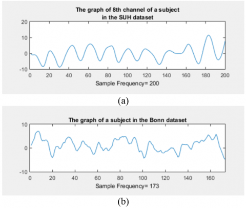
In Figure 8, 1-second EEG signal images from both datasets used in the study are given. When the signals are examined, the approximate frequency value of the signals in Figure 8.a) can be easily observed as 8. This signal points to the Theta wave range in Table 1. On the other hand, it was observed in Figure 8.b) that the average frequency value of the signals is greater than 8. It can be said that there is no SW in this signal given as an example in the Bonn dataset.
Since the SUH dataset does not include any normal EEG record without any disease diagnosis, normal EEG records in the public Bonn dataset were utilized to determine the accuracy and reliability of the method. For this reason, these two datasets were used to determine the success of the method implemented. The characteristics of this dataset are given in Table 7.
Table 5. The information of data files in routine EEG
|
Subject# |
Page# |
File Size |
|
suh-01 |
53 |
159000 |
|
suh-02 |
61 |
183000 |
|
suh-03 |
64 |
192000 |
|
suh-04 |
57 |
171000 |
|
suh-05 |
59 |
177000 |
|
suh-06 |
48 |
144000 |
|
suh-07 |
59 |
177000 |
|
suh-08 |
60 |
180000 |
|
suh-09 |
57 |
171000 |
|
suh-10 |
54 |
162000 |
|
suh-11 |
58 |
174000 |
|
suh-12 |
56 |
168000 |
|
suh-13 |
57 |
171000 |
|
suh-14 |
58 |
174000 |
|
suh-15 |
60 |
180000 |
|
suh-16 |
59 |
177000 |
|
suh-17 |
54 |
162000 |
|
suh-18 |
61 |
183000 |
|
suh-19 |
57 |
171000 |
|
suh-20 |
58 |
174000 |
|
suh-21 |
57 |
171000 |
|
suh-22 |
59 |
177000 |
|
Average |
57.55 |
172636.36 |
|
Min |
48 |
144000 |
|
Max |
64 |
192000 |
Table 6. Pivot table of the SUH dataset
|
Pages# |
The number of repetitions |
|
48 |
1 |
|
53 |
1 |
|
54 |
2 |
|
56 |
1 |
|
57 |
5 |
|
58 |
3 |
|
59 |
4 |
|
60 |
2 |
|
61 |
2 |
|
64 |
1 |
|
Grand Total 22 |
|
Figure 7. Graph of the probability plot of normal distribution in the SUH dataset (Each page consists of 3000 samples as 200 sample rates x 15 seconds)
Table 7. Overview of Bonn dataset (Only dataset A was used in the study)
|
|
Healthy Individuals |
Epilepsy Individuals |
|||
|
Dataset |
A |
B |
C |
D |
E |
|
State |
Awake with eyes open |
Awake with eyes closed |
Seizure-free |
Seizure-free |
Seizure activity |
|
Electrode type |
Surface |
Surface |
Intracranial |
Intracranial |
Intracranial |
|
Electrode placement |
10/20 international system |
10/20 international system |
10/20 opposite to epileptogenic zone |
Within epileptogenic zone |
Within epileptogenic zone |
As shown in the table, the records in the Bonn dataset are obtained in five different ways. The sampling frequency of the records is 173.61 Hz, and each dataset consists of 100 records. In this dataset, a low pass filter of 40 Hz is applied for the first step of the analysis [49]. There are five different records encoded with A, B, C, D, and E, as it is seen obviously in the table. It is the Bonn dataset A (eyes open and scalp EEG) that is appropriate for the recording properties of the data in the SUH dataset. Accordingly, the reliability of the method performed using only the A dataset was tested in this study.
Figure 8. Signals in the SUH and Bonn dataset a) 1 second EEG signal display in SUH dataset, b) 1 second EEG signal display in Bonn dataset
General background slowing (theta and delta frequency ranges) is a normal finding on EEG when it signifies developmental slowing or the development of lethargy and sleep activity in children, adolescents, and some young adults. The background EEG is generally normal in patients with epilepsy [50]. On the other hand, general or focal background slowing can be seen in the EEG records of epilepsy patients. When it is not diagnosed accurately, patients with psychogenic non-epileptic seizures (PNES) encounter serious and multifaceted problems such as delay in starting the correct treatment, the long-term financial burden of antiepileptic drugs, and possible side effects.
An epileptic seizure manifests itself with sudden changes in sensory-motor functions, behaviour, memory, and consciousness. In general, the way the seizure manifests itself behaviourally varies depending on the localization and area of the affected brain area [51]. Epilepsy classification is most frequently made according to this clinical situation. According to this classification, epileptic seizures are examined in two parts: partial seizures affecting only a certain part of the brain and not always accompanied by loss of consciousness, and generalized seizures affecting the whole brain, always with loss of consciousness [52]. Etiologically, epilepsies are examined in two groups as primary or idiopathic and secondary epilepsies [53].
The main question that needs to be answered in patients coming to the clinic with loss of consciousness is whether the situation is an epileptic seizure. Since the seizure has already stopped when the patient is taken to the hospital, the most critical information in distinguishing this can be gathered from the patient or the eyewitnesses present during the loss of consciousness. In cases where anamnesis cannot be taken adequately, it becomes difficult to make a differential diagnosis to the patient. Besides, having a single seizure does not mean that a person has epilepsy. Epilepsy, as mentioned earlier, is a disease that occurs without any triggering cause and is defined by recurrent (two or more) seizures [54]. For this reason, it is critically essential to consider all epileptic activities that can be observed in EEG recordings. The main focus of recent studies has been on transient activities, which are signs of epileptic activity. However, the detection of slow waves is at least as critical as the detection of transient activities [19]. That being the case, a new MPP-based method has been developed to determine the relevance of SWs, which are the signs of EEG anomalies, with epilepsy and other neurological diseases, and to determine which regions of the brain are frequently detected (focal, lateralized, generalized).
For a better understanding of the working principle of the method, all examples are explained using a single data (suh-01) in the SUH dataset. The image of a 15-second EEG recording obtained from subject suh-01 data is shown in Figure 9. Even though the ground activities generally include alpha waves, SWs are encountered in some channels, as can be seen in the Figure 9. Photic Stimulation is one of the activation methods applied during routine EEG recording. Eyelid myoclonus, generalized myoclonic jerks, absence seizures, generalized tonic clonic seizures, focal seizures, and more rarely tonic versive seizures and focal asymmetric myoclonic seizures can be triggered by photic stimulation [55]. In addition, the emergence of generalized discharges consisting of spike-slow wave, sharp wave-slow wave and multiple spike-slow wave elements in epilepsies generalized with photic stimulation becomes easier. In this technique, a bright light stimulus flashing at different frequencies for 5-10 seconds is applied to a patient from a distance of 30 cm with eyes open and closed. The blue line in Figure 9 and the blue line shown at the bottom (photic stimulation) was applied for 10 seconds. The fact that this blue line continues straight means that photic stimulation is not applied.
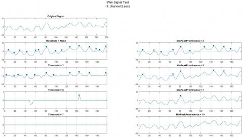
Detecting background activities that indicate the anomaly is quite significant for diagnosis and treatment. Therefore, the signal that Discrete Wavelet Transform (DWT) or any pass filter (low pass, high pass, etc.) is not applied has been examined with threshold and MPP. For the signal analysis here, various studies have been conducted on the peak values of the original signal and the peaks obtained after applying the threshold and MPP. That's why the focus has been on the signals belonging to all channels in the second of the subject suh-01 dataset. First of all, 1st and 2nd channels of these signals in the 2nd second were examined. Various trials were carried out by giving different values for Threshold and MPP. As it is seen in Figure 10, the peaks and peak numbers obtained with both techniques are indicated. All peak numbers (original signal, threshold, and MPP) obtained as a result of the trials are taken into a matrix. Afterward, the peak numbers obtained by threshold and MPP were subtracted from the original peak numbers and the differences between them were analysed. Analysing the obtained differences, it was determined that the channels with the least subtraction result had SW as given in Figure 10. The differences between all the peak numbers in each dataset were obtained through the program written in the Matlab program.
The numerically obtained differences between the peak numbers of the original signal obtained before any processing and the peaks obtained as a result of the threshold and MPP are shown in Table 8. The difference 1, difference 2 and difference 3 indicate the values obtained by the MPP method, while the difference 4, difference 5 and difference 5 indicate the values obtained by the Threshold method, respectively. In Table 8, the values where the difference between the peak numbers of the original signal and the peak numbers obtained with the threshold and MPP techniques is 3 and below 3 are marked with a green background colour. These values marked signify possible SW. Examining the table, when MPP 2 and 5 values were given, 8 and 4 SWs were found, respectively. On the other side, 3 and 1 SWs were found for threshold 2 and 5, respectively, but no SW was found for the value 7. Signals that may be SWs were almost never detected, especially in trials with the threshold. As it is shown in the table, when the value 7 for MPP is given, SWs marked manually by a neurologist were found to be high. That's why the value 7 was taken as the basis for the MPP based method implemented, and this value was used on all the next dataset. SUH and Bonn datasets were used to test the reliability and accuracy of the MPP method.
To determine which channels and on which pages the SWs are seen frequently, the data were processed page by page. Besides, it was determined in which channels it was frequently seen by taking the average SWs value for each channel. In this way, it was determined in which areas of the brain the SWs are seen or whether they are seen in all (focal, lateralized, and generalized).
Statistical measures of the performance, commonly used in scientific studies, were used to evaluate the success of the method. As it is known, the confusion matrix is one of the easiest and well-known methods used to interpret the success of classifiers [56]. This confusion matrix provides us with detailed information regarding correct and incorrect predictions in classification. In this method that generally evaluates the performance of data in the form of matrixes, there are four possible results: True Positive (TP), True Negative (TN), False Positive (FP), and False Negative (FN). Explanations of these possible results are given in Table 9 [57, 58].
Figure 9. 18-channel EEG recording (only 15 sec) of the subject suh-01. Generally, the ground activity is well developed in the posterior areas of the hemispheres and includes 8-13 Hz alpha waves. However, SW is observed in some of the channels marked
Figure 10. Peak detection trials of the signals in the 2nd second of channels 1 and 2 of the subject suh-01. a) 1. Channel on 2nd second, b) 2. Channel on 2nd second
The performance of a classifier is assessed by statistical parameters such as Sensitivity (SEN), specificity (SPE), and classification accuracy (ACC) (Eqns. (1), (2), and (3)).
SEN=TP/(TP+FN) (1)
SPE=TN/(TN+FP) (2)
ACC= (TP+TN)/(TP+TN+FP+FN) (3)
Examining the classifier success (ACC) alone is not always adequate to evaluate the success of a system. Especially in imbalanced datasets, it will be beneficial to examine the parameters of precision (Eq. (4)) and F-score (Eq. (5)) together with these parameters. The Positive Predicted Value (PPV) or Precision value provides information regarding how many of those identified as patients are actually sick, and the F-score (also F-measure or F1-score) is used to calculate the truth of a test and it balances the use of precision. The F-score value can provide the measurement of a test's performance in a more realistic way through both precision and recall.
PPV=TP/(TP+FP) (4)
F-score=2TP/(2TP+FP+FN) (5)
Table 8. The peak numbers obtained in the 2nd second of all channels of the subject suh-01 (Available/No Available (A/N))
|
Channel Name |
SWs (A/N) |
The number of Original Peaks (all channel - 2 second) Threshold=None |
MPP |
Threshold |
||||||||||
|
=2 |
Difference 1 |
=5 |
Difference 2 |
=7 |
Difference 3 |
=2 |
Difference 4 |
=5 |
Difference 5 |
=7 |
Difference 6 |
|||
|
Fp1-F7 |
N |
15 |
10 |
5 |
5 |
10 |
1 |
14 |
11 |
4 |
1 |
14 |
0 |
15 |
|
F7-T3 |
N |
14 |
10 |
4 |
5 |
9 |
3 |
11 |
13 |
1 |
5 |
9 |
1 |
13 |
|
T3-T5 |
N |
13 |
10 |
3 |
6 |
7 |
5 |
8 |
10 |
3 |
5 |
8 |
2 |
11 |
|
T5-O1 |
A |
10 |
10 |
0 |
10 |
0 |
6 |
4 |
10 |
0 |
6 |
4 |
2 |
8 |
|
Fp1-F3 |
N |
13 |
10 |
3 |
2 |
11 |
1 |
12 |
8 |
5 |
1 |
12 |
0 |
13 |
|
F3-C3 |
N |
13 |
11 |
2 |
6 |
7 |
3 |
10 |
13 |
0 |
3 |
10 |
0 |
13 |
|
C3-P3 |
N |
13 |
10 |
3 |
7 |
6 |
5 |
8 |
|
13 |
4 |
9 |
2 |
11 |
|
P3-O1 |
A |
11 |
11 |
0 |
9 |
2 |
9 |
2 |
|
11 |
8 |
3 |
7 |
4 |
|
FZ-CZ |
N |
12 |
11 |
1 |
9 |
3 |
3 |
9 |
|
12 |
2 |
10 |
1 |
11 |
|
CZ-PZ |
N |
13 |
9 |
4 |
7 |
6 |
4 |
9 |
|
13 |
4 |
9 |
1 |
12 |
|
Fp2-F8 |
N |
15 |
6 |
9 |
3 |
12 |
3 |
12 |
|
15 |
7 |
8 |
6 |
9 |
|
F8-T4 |
N |
12 |
11 |
1 |
8 |
4 |
6 |
6 |
|
12 |
6 |
6 |
2 |
10 |
|
T4-T6 |
N |
13 |
11 |
2 |
9 |
4 |
7 |
6 |
|
13 |
7 |
6 |
2 |
11 |
|
T6-O2 |
N |
13 |
10 |
3 |
7 |
6 |
6 |
7 |
|
13 |
6 |
7 |
4 |
9 |
|
Fp2-F4 |
N |
14 |
8 |
6 |
4 |
10 |
2 |
12 |
|
14 |
4 |
10 |
1 |
13 |
|
F4-C4 |
N |
11 |
11 |
0 |
9 |
2 |
5 |
6 |
|
11 |
5 |
6 |
0 |
11 |
|
C4-P4 |
N |
13 |
9 |
4 |
8 |
5 |
8 |
5 |
|
13 |
8 |
5 |
3 |
10 |
|
P4-O2 |
A |
12 |
11 |
1 |
10 |
2 |
10 |
2 |
|
12 |
11 |
1 |
8 |
4 |
Table 9. Possible results on confusion matrix
|
Predicted Values |
|||
|
Actual Values |
|
0 |
1 |
|
0 |
TN (Telling not sick to those who are not sick) |
FP (Telling sick to those who are not sick) |
|
|
1 |
FN (Telling not sick to those who are sick) |
TP (Telling sick to those who are sick) |
|
The average of ACC values obtained with the confusion matrix found for the SUH dataset is given in Table 10. Comparing the average ACC values obtained by the method performed with clinical findings, it was found that there was a high rate of SWs in places where the average value was 1 and greater than 1 (channel numbers with SWs are marked in the relevant table for each data). For this reason, those with an average ACC value less than 1 were not taken into account.
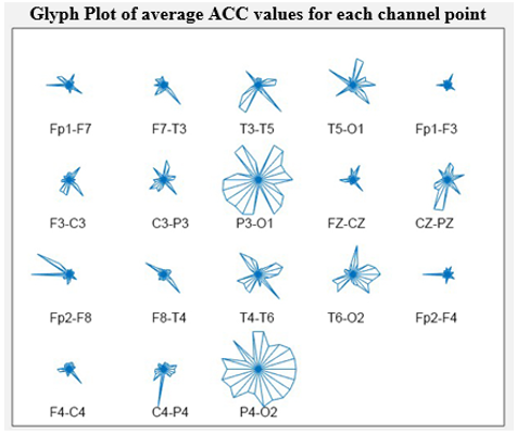
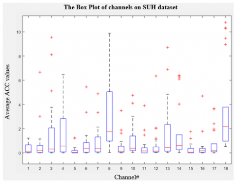
For a better analysis, the average ACC values given in Table 11 were plotted with glyphplot (Figure 11). In this way, it is better to analyse which channels have more SWs by examining these values visually for each channel. The graph shows that the channels with the most SWs are the 8th (P3-O1) and 18th (P4-O2) channels. However, in general, a considerable number of SWs were detected in the 3rd (T3-T5), 4th (T5-O1), 10th (CZ-PZ), 13th (T4-T6), and 14th (T6-O2) channels. When the electrode connection points of the channels where SWs are most frequently seen were examined, it was found that they were in both hemispheres (both right and left), around the occipital area, that is, in the posterior part of the skull (Figure 12). This indicates that such SWs are observed in the posterior areas of the brain, particularly in the temporal, parietal, and occipital regions.
Table 10. Confusion matrix for the SUH dataset
|
suh-01 |
0 |
1 |
|
suh-02 |
0 |
1 |
|
suh-03 |
0 |
1 |
|
suh-04 |
0 |
1 |
|
|
0 |
454 |
57 |
511 |
0 |
165 |
14 |
179 |
0 |
535 |
19 |
554 |
0 |
912 |
16 |
928 |
|
1 |
13 |
430 |
443 |
1 |
8 |
911 |
919 |
1 |
15 |
583 |
598 |
1 |
7 |
91 |
98 |
|
|
467 |
487 |
954 |
|
173 |
925 |
1098 |
|
550 |
602 |
1152 |
|
919 |
107 |
1026 |
|
|
|
|
|
|
|
|
|
|
|
|
|
|
|
|
|
|
suh-05 |
0 |
1 |
|
suh-06 |
0 |
1 |
|
suh-07 |
0 |
1 |
|
suh-08 |
0 |
1 |
|
|
0 |
573 |
25 |
598 |
0 |
655 |
19 |
674 |
0 |
688 |
18 |
706 |
0 |
788 |
17 |
805 |
|
1 |
14 |
450 |
464 |
1 |
23 |
167 |
190 |
1 |
15 |
341 |
356 |
1 |
11 |
264 |
275 |
|
|
587 |
475 |
1062 |
|
678 |
186 |
864 |
|
703 |
359 |
1062 |
|
799 |
281 |
1080 |
|
|
|
|
|
|
|
|
|
|
|
|
|
|
|
|
|
|
suh-09 |
0 |
1 |
|
suh-10 |
0 |
1 |
|
suh-11 |
0 |
1 |
|
suh-12 |
0 |
1 |
|
|
0 |
872 |
25 |
897 |
0 |
654 |
13 |
667 |
0 |
912 |
8 |
920 |
0 |
712 |
35 |
747 |
|
1 |
6 |
123 |
129 |
1 |
12 |
293 |
305 |
1 |
8 |
116 |
124 |
1 |
9 |
252 |
261 |
|
|
878 |
148 |
1026 |
|
666 |
306 |
972 |
|
920 |
124 |
1044 |
|
721 |
287 |
1008 |
|
|
|
|
|
|
|
|
|
|
|
|
|
|
|
|
|
|
|
|
|
|
|
|
|
|
|
|
|
|
|
|
|
|
|
suh-13 |
0 |
1 |
|
suh-14 |
0 |
1 |
|
suh-15 |
0 |
1 |
|
suh-16 |
0 |
1 |
|
|
0 |
858 |
15 |
873 |
0 |
865 |
7 |
872 |
0 |
415 |
37 |
452 |
0 |
642 |
24 |
666 |
|
1 |
21 |
132 |
153 |
1 |
17 |
155 |
172 |
1 |
8 |
620 |
628 |
1 |
19 |
377 |
396 |
|
|
879 |
147 |
1026 |
|
882 |
162 |
1044 |
|
423 |
657 |
1080 |
|
661 |
401 |
1062 |
|
|
|
|
|
|
|
|
|
|
|
|
|
|
|
|
|
|
suh-17 |
0 |
1 |
|
suh-18 |
0 |
1 |
|
suh-19 |
0 |
1 |
|
suh-20 |
0 |
1 |
|
|
0 |
629 |
35 |
664 |
0 |
1034 |
14 |
1048 |
0 |
805 |
24 |
829 |
0 |
203 |
22 |
225 |
|
1 |
30 |
278 |
308 |
1 |
9 |
41 |
50 |
1 |
11 |
186 |
197 |
1 |
7 |
812 |
819 |
|
|
659 |
313 |
972 |
|
1043 |
55 |
1098 |
|
816 |
210 |
1026 |
|
210 |
834 |
1044 |
|
|
|
|
|
|
|
|
|
|
|
|
|
|
|
|
|
|
suh-21 |
0 |
1 |
|
suh-22 |
0 |
1 |
|
|
|
|
|
|
|
|
|
|
0 |
645 |
41 |
686 |
0 |
988 |
8 |
996 |
|
|
|
|
|
|
|
|
|
1 |
24 |
316 |
340 |
1 |
14 |
52 |
66 |
|
|
|
|
|
|
|
|
|
|
669 |
357 |
1026 |
|
1002 |
60 |
1062 |
|
|
|
|
|
|
|
|
Table 11. Average of SWs numbers found for all channels in the SUH dataset
|
Subject# |
Fp1-F7 |
F7-T3 |
T3-T5 |
T5-O1 |
Fp1-F3 |
F3-C3 |
C3-P3 |
P3-O1 |
FZ-CZ |
CZ-PZ |
Fp2-F8 |
F8-T4 |
T4-T6 |
T6-O2 |
Fp2-F4 |
F4-C4 |
C4-P4 |
P4-O2 |
|
1 |
0.1 |
0.1 |
3.5 |
5.0 |
0.0 |
0.7 |
1.7 |
8.1 |
0.5 |
0.7 |
0.2 |
0.5 |
4.2 |
6.3 |
0.1 |
0.2 |
1.8 |
9.0 |
|
2 |
1.1 |
1.1 |
5.1 |
3.6 |
1.2 |
1.0 |
3.3 |
7.6 |
1.9 |
4.8 |
1.5 |
2.1 |
6.9 |
6.4 |
1.8 |
1.8 |
3.7 |
10.3 |
|
3 |
0.7 |
0.4 |
2.1 |
3.1 |
0.3 |
0.9 |
1.0 |
6.5 |
0.1 |
1.0 |
0.4 |
1.2 |
4.8 |
4.0 |
0.1 |
0.4 |
0.8 |
9.5 |
|
4 |
0.0 |
0.0 |
0.0 |
0.0 |
0.0 |
0.4 |
0.1 |
1.0 |
0.0 |
0.1 |
0.0 |
0.1 |
0.1 |
0.1 |
0.0 |
0.1 |
0.1 |
0.9 |
|
5 |
1.2 |
0.1 |
0.5 |
2.8 |
1.2 |
0.4 |
1.3 |
4.5 |
1.6 |
1.4 |
0.4 |
0.2 |
0.4 |
1.1 |
0.7 |
0.5 |
0.4 |
2.8 |
|
6 |
0.1 |
0.0 |
0.2 |
1.4 |
0.0 |
0.2 |
0.9 |
0.1 |
0.2 |
0.8 |
0.0 |
0.1 |
0.0 |
1.5 |
0.0 |
0.1 |
0.2 |
2.0 |
|
7 |
0.1 |
0.6 |
0.4 |
0.2 |
0.2 |
0.4 |
0.1 |
1.6 |
0.9 |
0.7 |
0.2 |
0.1 |
1.0 |
0.9 |
0.4 |
0.3 |
0.0 |
3.8 |
|
8 |
0.1 |
0.4 |
0.2 |
0.8 |
0.0 |
0.1 |
0.3 |
5.1 |
0.1 |
0.4 |
0.0 |
0.4 |
2.2 |
0.5 |
0.0 |
0.4 |
0.1 |
1.0 |
|
9 |
0.2 |
0.1 |
0.5 |
0.0 |
0.1 |
0.0 |
0.4 |
1.0 |
0.1 |
0.3 |
0.3 |
0.1 |
0.8 |
0.0 |
0.0 |
0.1 |
0.1 |
1.0 |
|
10 |
1.2 |
0.7 |
0.1 |
2.8 |
0.0 |
0.3 |
0.1 |
0.4 |
0.1 |
0.2 |
3.9 |
2.0 |
0.7 |
0.7 |
0.0 |
0.2 |
0.4 |
1.2 |
|
11 |
0.0 |
0.0 |
0.0 |
0.3 |
0.0 |
0.0 |
0.0 |
1.4 |
0.0 |
0.1 |
0.0 |
0.0 |
0.0 |
0.4 |
0.0 |
0.0 |
0.0 |
2.7 |
|
12 |
1.1 |
0.3 |
0.0 |
0.1 |
0.4 |
0.2 |
0.4 |
1.7 |
0.6 |
0.2 |
1.9 |
0.1 |
0.0 |
0.1 |
1.2 |
0.4 |
0.3 |
1.5 |
|
13 |
0.0 |
0.0 |
0.1 |
0.0 |
0.0 |
0.1 |
0.1 |
0.9 |
0.1 |
0.3 |
0.1 |
0.0 |
0.5 |
0.5 |
0.0 |
0.2 |
0.1 |
0.9 |
|
14 |
0.0 |
0.1 |
0.4 |
0.5 |
0.0 |
0.0 |
0.4 |
1.0 |
0.0 |
0.3 |
0.1 |
0.0 |
0.4 |
0.4 |
0.1 |
0.0 |
0.2 |
0.8 |
|
15 |
0.2 |
3.0 |
8.1 |
0.7 |
0.2 |
3.4 |
2.1 |
9.9 |
0.1 |
3.0 |
0.7 |
1.1 |
4.8 |
6.1 |
0.2 |
0.0 |
3.6 |
10.8 |
|
16 |
0.1 |
0.7 |
3.8 |
0.4 |
0.0 |
1.4 |
1.3 |
4.9 |
0.2 |
4.1 |
0.0 |
0.2 |
2.3 |
0.1 |
0.0 |
0.3 |
0.2 |
3.0 |
|
17 |
0.0 |
0.2 |
0.1 |
0.2 |
0.2 |
0.9 |
0.3 |
2.2 |
0.1 |
1.9 |
0.5 |
0.1 |
0.0 |
0.3 |
0.4 |
0.3 |
2.4 |
1.5 |
|
18 |
0.1 |
0.0 |
0.0 |
0.0 |
0.0 |
0.0 |
0.0 |
0.0 |
0.0 |
0.0 |
0.0 |
0.0 |
0.1 |
0.1 |
0.0 |
0.0 |
0.0 |
0.5 |
|
19 |
0.1 |
0.2 |
0.6 |
0.9 |
0.1 |
0.0 |
0.1 |
4.0 |
0.1 |
0.3 |
0.0 |
0.1 |
0.4 |
1.0 |
0.0 |
0.0 |
0.1 |
3.5 |
|
20 |
0.4 |
6.7 |
9.6 |
6.5 |
0.0 |
5.4 |
4.9 |
9.5 |
3.5 |
4.7 |
0.3 |
6.3 |
8.7 |
6.4 |
0.1 |
4.7 |
1.9 |
10.3 |
|
21 |
0.9 |
0.4 |
0.1 |
0.8 |
0.4 |
0.5 |
0.3 |
1.8 |
0.1 |
0.4 |
0.4 |
0.5 |
0.3 |
1.0 |
0.4 |
0.2 |
0.4 |
2.4 |
|
22 |
0.0 |
0.0 |
0.0 |
0.1 |
0.0 |
0.0 |
0.0 |
0.2 |
0.0 |
0.0 |
0.0 |
0.0 |
0.1 |
0.3 |
0.0 |
0.0 |
0.2 |
0.6 |
Figure 11. The indication of the peak averages monitored by channels through glyhplot for the SUH dataset
The number of SWs seen in the channels is given in Table 12. Examining the frequency values 6 and higher than 6 in the table, it was determined that the channels with the most SWs are T3-T5, T5-O1, P3-O1, CZ-PZ, T4-T6, T6-O2, and P4-O2.
Figure 12. The indication of the areas where SWs are most frequently seen in the electrode connection (channels marked in blue are the channels with the most SWs), according to the results obtained (SUH dataset)
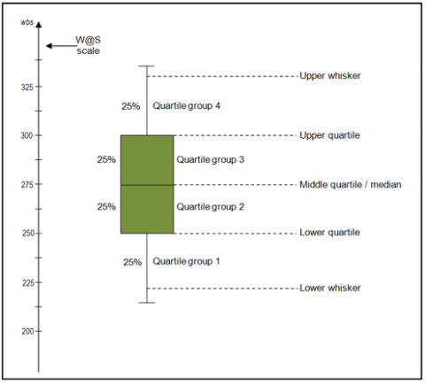
Also, all SWs found for the SUH dataset were examined with a box plot on a channel basis. A box plot (also known as box and whisker plot) is a type of chart used to visually indicate the distribution of quantitative data, the distributions and skewness between variables or between levels of a categorical variable. The summary of a dataset consists of five parts: minimum score, first (lower) quarter, median, third (upper) quarter, and maximum score (Figure 13).
Table 12. Frequency of SWs by channels for the SUH dataset (numerically)
|
No. of Channel |
Channel Name |
Count of Channel Frequency |
|
1 |
Fp1-F7 |
4 |
|
2 |
F7-T3 |
3 |
|
3 |
T3-T5 |
6 |
|
4 |
T5-O1 |
7 |
|
5 |
Fp1-F3 |
2 |
|
6 |
F3-C3 |
3 |
|
7 |
C3-P3 |
7 |
|
8 |
P3-O1 |
15 |
|
9 |
FZ-CZ |
3 |
|
10 |
CZ-PZ |
7 |
|
11 |
Fp2-F8 |
3 |
|
12 |
F8-T4 |
5 |
|
13 |
T4-T6 |
8 |
|
14 |
T6-O2 |
8 |
|
15 |
Fp2-F4 |
2 |
|
16 |
C4-C4 |
2 |
|
17 |
C4-P4 |
5 |
|
18 |
P4-O2 |
16 |
|
|
Grand Total |
106 |
Figure 13. Boxplot [59]
In the box plot, the analysis is made according to the location of the median on the box. If the median is in the middle of the box and its whiskers are equidistant from both sides of the box, the distribution is symmetrical. If the median is closer to the bottom of the box and the whisker is shorter at the lower end of the box, the distribution is positively skewed. Finally, if the median is closer to the top of the box and the whisker is shorter at the upper end of the box, the distribution is negatively skewed. Considering these characteristics of the box plot, distributions and distortions between average ACC values can be visually analysed. Examining the variables given in Figure 14, it is observed that all the median values are close to the bottom of the box, and again they are quite short on their whiskers. Consequently, it can be said that the distribution is positively skewed. Besides, examining the graphic in general, it is quite obviously observed that the frequency of SWs is the highest in channels 3, 4, 8, 13, and 18. Interquartile range give us information about how the data is dispersed among each sample. In other words, as the box gets longer, the data shows more dispersal. On the other hand, the data is dispersed less as the box get smaller. When we look at Figure 14, the box showing the 8th channel is longer than the other boxes. In this case, it is seen that there are more SWs dispersals on this channel. The whiskers at the ends of each box give us information about the general spread. Looking at the whiskers in this figure, a wider spread was observed in channels 4 and 13, especially in the 8th channel. In other words, the data are observed as more dispersed in these channels.
Besides, it was examined in which areas of the brain SWs are seen more frequently, according to the results. The results of the analysis achieved in this context are given in Table 13. Examining the table, it was observed that slow waves emerge as generalized rather than focal or lateralized. It was determined that especially the multifocal occurrence, coded as D (at least 2 focus, each in different hemispheres), is more than the others. That being the case, it was determined that SWs are observed as multifocal in EEG recordings and, as discussed earlier, they are most frequently observed in the occipital area that includes both sides of the brain.
Figure 14. The indication of the average ACC values obtained with Boxplot (SUH dataset)
Table 13. The frequencies of SW values by the brain regions for the SUH dataset
|
Code |
Brain region/hemisphere |
Frequency of SW |
|
A |
No-SWs or any SWs |
4 |
|
B |
one region - one focus |
2 |
|
C |
one hemisphere |
None |
|
D |
multifocal (at least 2 focus, each in different hemisphere) |
15 |
|
E |
multifocal (at least 2 focus, each in same hemisphere) |
None |
|
F |
generalized |
1 |
|
|
Total Data |
22 |
Statistical performance measurement results are presented in Table 14 in its most general form. All TP, TN, FP, FN values observed for the SUH dataset, and the results of the classifier metrics obtained with these values are seen in detail. The lowest ACC value is 92.7%, and the highest ACC value is 98.5%. Looking at the PPV values in the table, the rate of correct detection was determined as 90.9% of those determined as SW. It was observed that the method performed according to the results has a high rate of success.
Figure 15. The graph of ACC on the SUH dataset
The main reason for using the F-Score value is not to make an incorrect model selection in unevenly distributed datasets. Besides, F-Score is a significant statistical metric when a measurement metric that includes not only FN or FP but also all error costs is needed. When the F1 score is 1, the model is considered perfect, and when it is 0, it is considered unsuccessful. Looking at Table 14, it is seen that F-score values are very close to 1 (average 92%).
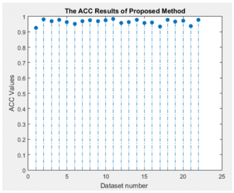
As it is seen in Figure 15, the classification success achieved for each data (22 subjects) is generally above 90%. The general average ACC value is 96.5% (Table 15). The method performed according to these results has a high rate of success in detecting SWs.
The results achieved were analyzed graphically with polynomial fitting (Figure 16). The curve fitting process was conducted with the Linear model Ploy3. As can be seen in the Figure 16, some data such as suh-06, suh-09, and suh-11 stay out of the fitting curve. However, most of the data collected as a result of the best model and the curve fitting process are appropriate for the model. Looking at the Root Mean Square Error (RMSE) value of the method performed, it has a small error rate of 0.01598.
The method performed on the second dataset (Bonn dataset) was implemented using the same values (7 value for MPP and average <=3). All average SW values obtained on the Bonn dataset are presented in Table 16. The averages of 1 and above 1 from the average SW values obtained for the SUH dataset were taken into account. Channels above 1 and 1 in the Bonn dataset must have SWs. However, when the table is examined, all the average values are below 1. This proves that there is no SW in the Bonn dataset (normal data - A) used in the study. Consequently, thanks to the method performed, while the SUH dataset had a high SW rate of 96.5%, a 100% success rate (ACC) was achieved in the Bonn dataset without SW.
Table 14. Experimental results using the proposed method on the SUH dataset (PPV, SEN, SPE, F-score, ACC)
|
Subject# |
TN |
FP |
FN |
TP |
PPV (%) |
SEN (%) |
SPE (%) |
F-score (%) |
ACC (%) |
|
1 |
454 |
57 |
13 |
430 |
88.3 |
97.1 |
88.8 |
92.5 |
92.7 |
|
2 |
165 |
14 |
8 |
911 |
98.5 |
99.1 |
92.2 |
98.8 |
98.0 |
|
3 |
535 |
19 |
15 |
583 |
96.8 |
97.5 |
96.6 |
97.2 |
97.0 |
|
4 |
912 |
16 |
7 |
91 |
85.0 |
92.9 |
98.3 |
88.8 |
97.8 |
|
5 |
573 |
25 |
14 |
450 |
94.7 |
97.0 |
95.8 |
95.8 |
96.3 |
|
6 |
655 |
19 |
23 |
167 |
89.8 |
87.9 |
97.2 |
88.8 |
95.1 |
|
7 |
688 |
18 |
15 |
341 |
95.0 |
95.8 |
97.5 |
95.4 |
96.9 |
|
8 |
788 |
17 |
11 |
264 |
94.0 |
96.0 |
97.9 |
95.0 |
97.4 |
|
9 |
872 |
25 |
6 |
123 |
83.1 |
95.3 |
97.2 |
88.8 |
97.0 |
|
10 |
654 |
13 |
12 |
293 |
95.8 |
96.1 |
98.1 |
95.9 |
97.4 |
|
11 |
912 |
8 |
8 |
116 |
93.5 |
93.5 |
99.1 |
93.5 |
98.5 |
|
12 |
712 |
35 |
9 |
252 |
87.8 |
96.6 |
95.3 |
92.0 |
95.6 |
|
13 |
858 |
15 |
21 |
132 |
89.8 |
86.3 |
98.3 |
88.0 |
96.5 |
|
14 |
865 |
7 |
17 |
155 |
95.7 |
90.1 |
99.2 |
92.8 |
97.7 |
|
15 |
415 |
37 |
8 |
620 |
94.4 |
98.7 |
91.8 |
96.5 |
95.8 |
|
16 |
642 |
24 |
19 |
377 |
94.0 |
95.2 |
96.4 |
94.6 |
96.0 |
|
17 |
629 |
35 |
30 |
278 |
88.8 |
90.3 |
94.7 |
89.5 |
93.3 |
|
18 |
1034 |
14 |
9 |
41 |
74.5 |
82.0 |
98.7 |
78.1 |
97.9 |
|
19 |
805 |
24 |
11 |
186 |
88.6 |
94.4 |
97.1 |
91.4 |
96.6 |
|
20 |
203 |
22 |
7 |
812 |
97.4 |
99.1 |
90.2 |
98.2 |
97.2 |
|
21 |
645 |
41 |
24 |
316 |
88.5 |
92.9 |
94.0 |
90.7 |
93.7 |
|
22 |
988 |
8 |
14 |
52 |
86.7 |
78.8 |
99.2 |
82.5 |
97.9 |
Table 15. Overall statistics in the SUH dataset
|
ACC (±std.dev.) |
SEN (±std.dev.) |
SPE (±std.dev.) |
Error rate |
||||||
|
96.5 |
± |
0.015785779 |
93.3 |
± |
0.054348636 |
96.1 |
± |
0.029663221 |
0.035 |
Figure 16. Graph of overall ACC on SUH dataset
Table 16. Average of SW on Bonn dataset
|
No. of records |
Average of SW |
No. of records |
Average of SW |
No. of records |
Average of SW |
No. of records |
Average of SW |
|
1 |
0.260869565 |
26 |
0.391304348 |
51 |
0.086956522 |
76 |
0.173913043 |
|
2 |
0.173913043 |
27 |
0.782608696 |
52 |
0.826086957 |
77 |
0.304347826 |
|
3 |
0.47826087 |
28 |
0.043478261 |
53 |
0.130434783 |
78 |
0.739130435 |
|
4 |
0.130434783 |
29 |
0.086956522 |
54 |
0.217391304 |
79 |
0.173913043 |
|
5 |
0.217391304 |
30 |
0.304347826 |
55 |
0.652173913 |
80 |
0 |
|
6 |
0.304347826 |
31 |
0 |
56 |
0.130434783 |
81 |
0.173913043 |
|
7 |
0.652173913 |
32 |
0.043478261 |
57 |
0.173913043 |
82 |
0.434782609 |
|
8 |
0.260869565 |
33 |
0.260869565 |
58 |
0.043478261 |
83 |
0.130434783 |
|
9 |
0 |
34 |
0.086956522 |
59 |
0.130434783 |
84 |
0.086956522 |
|
10 |
0.086956522 |
35 |
0.391304348 |
60 |
0.086956522 |
85 |
0.130434783 |
|
11 |
0 |
36 |
0.130434783 |
61 |
0.130434783 |
86 |
0 |
|
12 |
0.130434783 |
37 |
0.130434783 |
62 |
0.304347826 |
87 |
0.043478261 |
|
13 |
0.043478261 |
38 |
0.086956522 |
63 |
0.043478261 |
88 |
0.086956522 |
|
14 |
0.130434783 |
39 |
0.217391304 |
64 |
0.043478261 |
89 |
0.130434783 |
|
15 |
0.043478261 |
40 |
0.043478261 |
65 |
0.565217391 |
90 |
0.434782609 |
|
16 |
0.086956522 |
41 |
0.130434783 |
66 |
0.086956522 |
91 |
0.043478261 |
|
17 |
0 |
42 |
0 |
67 |
0.086956522 |
92 |
0.434782609 |
|
18 |
0.347826087 |
43 |
0.130434783 |
68 |
0.173913043 |
93 |
0.391304348 |
|
19 |
0 |
44 |
0.304347826 |
69 |
0.391304348 |
94 |
0.347826087 |
|
20 |
0.043478261 |
45 |
0.347826087 |
70 |
0 |
95 |
0.608695652 |
|
21 |
0 |
46 |
0.130434783 |
71 |
0.173913043 |
96 |
0.391304348 |
|
22 |
0.043478261 |
47 |
0.043478261 |
72 |
0.608695652 |
97 |
0.347826087 |
|
23 |
0.304347826 |
48 |
0.391304348 |
73 |
0 |
98 |
0.173913043 |
|
24 |
0.043478261 |
49 |
0.260869565 |
74 |
0.173913043 |
99 |
0.739130435 |
|
25 |
0.173913043 |
50 |
0.260869565 |
75 |
0.347826087 |
100 |
0 |
Epilepsy is a disease that necessitates long-term monitoring and treatment. The first step to be followed is to establish the correct diagnosis and decide whether drug therapy is needed. The diagnosis and classification of epilepsy depend primarily on the patient's past medical records and physical findings. Epilepsy may manifest itself in various clinical forms. Its clinical features, etiology, severity, prognosis, and other accompanying neurological findings are quite variable, so there might be challenges in making a differential diagnosis.
Epileptic seizures in epilepsy patients are not random events, but they are the products of highly complex dynamic brain networks developing over time [9]. Epileptic seizures negatively affect both the consciousness and memory states of patients and their motor and sensory functions. Besides, the patients' quality of life is considerably reduced because of the negative risks of anti-epileptic drugs [60]. Therefore, a correct analysis of EEG records will make a great contribution to the diagnosis. Computer-aided automatic EEG examinations are required because of reasons such as undesirable situations occurring during long EEG recordings, a long examination by the neurologist, and lack of time for EEG examination. Within this scope, many studies have been conducted in the literature, particularly on the detection of transient activities. SW activities, mostly examined in sleep EEG, have not been emphasized adequately, though. Due to these reasons, a new method for detecting SWs has been developed in this study. The results of the study were compared with clinical information and the opinion of the specialist physician was received. When the results obtained with the method performed were compared with manual examinations, a high degree of accuracy was found. A further study in which both transient activities and background activities can be evaluated together will be beneficial to examine the effects and successes on online records other than retrospective records.
This study was achieved during Sema Yıldırım's doctoral thesis in Konya Technical University, Graduate Education Institute. We would like to thank the healthcare professionals in the neurology department who contributed to the preparation of the study for their knowledge and contributions.
[1] Duffy, F.H., Iyer, V.G. Surwillo, W.W., Gevins, A. (1990). Clinical electroencephalography and topographic brain mapping. Journal of Clinical Neurophysiology, 7(2): 296-299.
[2] Sharma, R., Pachori, R.B. (2015). Classification of epileptic seizures in EEG signals based on phase space representation of intrinsic mode functions. Expert Systems with Applications, 42(3): 1106-1117. https://doi.org/10.1016/j.eswa.2014.08.030
[3] Beghi, E., Berg, A., Carpio, A., Forsgren, L., Hesdorffer, D.C., Hauser, W.A., Tomson, T. (2005). Comment on epileptic seizures and epilepsy: definitions proposed by the International League Against Epilepsy (ILAE) and the International Bureau for Epilepsy (IBE). Epilepsia, 46(10): 1698-1699. https://doi.org/10.1111/j.1528-1167.2005.00273_1.x
[4] Berg, A.T., Berkovic, S.F., Brodie, M.J., Buchhalter, J., Cross, J.H., van Emde Boas, W., Scheffer, I.E. (2010). Revised terminology and concepts for organization of seizures and epilepsies. Report of the ILAE Commission on Classification and Terminology, 2005-2009. https://doi.org/10.1111/j.1528-1167.2010.02522.x
[5] Fisher, R.S., Boas, W.V.E., Blume, W., Elger, C., Genton, P., Lee, P., Engel Jr, J. (2005). Epileptic seizures and epilepsy: Definitions proposed by the International League Against Epilepsy (ILAE) and the International Bureau for Epilepsy (IBE). Epilepsia, 46(4): 470-472. https://doi.org/10.1111/j.0013-9580.2005.66104.x
[6] Subasi, A. (2005). Epileptic seizure detection using dynamic wavelet network. Expert Systems with Applications, 29(2): 343-355. https://doi.org/10.1016/j.eswa.2005.04.007
[7] Song, Y., Zhang, J. (2013). Automatic recognition of epileptic EEG patterns via extreme learning machine and multiresolution feature extraction. Expert Systems with Applications, 40(14): 5477-5489. https://doi.org/10.1016/j.eswa.2013.04.025
[8] Adeli, H., Zhou, Z., Dadmehr, N. (2003). Analysis of EEG records in an epileptic patient using wavelet transform. Journal of Neuroscience Methods, 123(1): 69-87. https://doi.org/10.1016/S0165-0270(02)00340-0
[9] Valderrama, M., Alvarado, C., Nikolopoulos, S., Martinerie, J., Adam, C., Navarro, V., Le Van Quyen, M. (2012). Identifying an increased risk of epileptic seizures using a multi-feature EEG–ECG classification. Biomedical Signal Processing and Control, 7(3): 237-244. https://doi.org/10.1016/j.bspc.2011.05.005
[10] Menshawy, M.E., Benharref, A., Serhani, M. (2015). An automatic mobile-health based approach for EEG epileptic seizures detection. Expert Systems with Applications, 42(20): 7157-7174. https://doi.org/10.1016/j.eswa.2015.04.068
[11] Çakıl, D., İnanır, S., Baykan, H., Aygün, H., Kozan, R. (2013). Epilepsi ayırıcı tanısında psikojenik non-epileptik nöbetler. Göztepe Tıp Dergisi, 28(1): 41-47.
[12] Henry, Z., Thomas, R. (2012). Seizures and epilepsy: electrophysiological diagnosis. Epilepsy board Rev. Man., 1(2): 1-45.
[13] Wilson, S.B., Scheuer, M.L., Emerson, R.G., Gabor, A.J. (2004). Seizure detection: Evaluation of the Reveal algorithm. Clinical Neurophysiology, 115(10): 2280-2291. https://doi.org/10.1016/j.clinph.2004.05.018
[14] Wilson, S.B., Turner, C.A., Emerson, R.G., Scheuer, M.L. (1999). Spike detection II: automatic, perception-based detection and clustering. Clinical Neurophysiology, 110(3): 404-411. https://doi.org/10.1016/S1388-2457(98)00023-6
[15] Cabrerizo, M., Ayala, M., Goryawala, M., Jayakar, P., Adjouadi, M. (2012). A new parametric feature descriptor for the classification of epileptic and control EEG records in pediatric population. International Journal of Neural Systems, 22(2): 1250001. https://doi.org/10.1142/S0129065712500013
[16] Wienbruch, C., Moratti, S., Elbert, T., Vogel, U., Fehr, T., Kissler, J., Rockstroh, B. (2003). Source distribution of neuromagnetic slow wave activity in schizophrenic and depressive patients. Clinical Neurophysiology, 114(11): 2052-2060. https://doi.org/10.1016/S1388-2457(03)00210-4
[17] Su, B.L., Luo, Y., Hong, C.Y., Nagurka, M.L., Yen, C.W. (2015). Detecting slow wave sleep using a single EEG signal channel. Journal of Neuroscience Methods, 243: 47-52. https://doi.org/10.1016/j.jneumeth.2015.01.023
[18] Liu, H.S., Zhang, T., Yang, F.S. (2002). A multistage, multimethod approach for automatic detection and classification of epileptiform EEG. IEEE Transactions on Biomedical Engineering, 49(12): 1557-1566. https://doi.org/10.1109/TBME.2002.805477
[19] Ji, Z., Sugi, T., Goto, S., Wang, X., Ikeda, A., Nagamine, T., Nakamura, M. (2011). An automatic spike detection system based on elimination of false positives using the large-area context in the scalp EEG. IEEE Transactions on Biomedical Engineering, 58(9): 2478-2488. https://doi.org/10.1109/TBME.2011.2157917
[20] Husain, A., Tatum, W.O., Kaplan, P.W. (2008). Handbook of EEG interpretation. Demos Med.
[21] Karakis, I., Montouris, G.D., Otis, J.A., Douglass, L.M., Jonas, R., Velez-Ruiz, N., Espinosa, P.S. (2010). A quick and reliable EEG montage for the detection of seizures in the critical care setting. Journal of Clinical Neurophysiology, 27(2): 100-105. https://doi.org/10.1097/WNP.0b013e3181d649e4
[22] Scherg, M., Bast, T., Berg, P. (1999). Multiple source analysis of interictal spikes: Goals, requirements, and clinical value. Journal of Clinical Neurophysiology, 16(3): 214-224.
[23] Raz, J., Biggins, C., Turetsky, B., Fein, G. (1993). Frequency domain dipole localization: extensions of the method and applications to auditory and visual evoked potentials. IEEE Transactions on Biomedical Engineering, 40(9): 909-918.
[24] Binnie, C.D., Holder, D.S. (1999). Electroencephalography. Handb. Clin. Neurol., 72: 283-318.
[25] Wang, B., Wang, X., Ikeda, A., Nagamine, T., Shibasaki, H., Nakamura, M. (2014). Automatic reference selection for quantitative EEG interpretation: Identification of diffuse/localised activity and the active earlobe reference, iterative detection of the distribution of EEG rhythms. Medical Engineering & Physics, 36(1): 88-95. https://doi.org/10.1016/j.medengphy.2013.10.002
[26] https://www.electrical4u.com/eeg-measurement, accessed on 11 July 2020.
[27] Sela, M. (2002). Electroencephalography: An introductory Text and Atlas, 62(12).
[28] Pradhan, N., Dutt, D.N. (1993). A nonlinear perspective in understanding the neurodynamics of EEG. Computers in Biology and Medicine, 23(6): 425-442. https://doi.org/10.1016/0010-4825(93)90091-E
[29] Xie, S., Krishnan, S. (2013). Wavelet-based sparse functional linear model with applications to EEGs seizure detection and epilepsy diagnosis. Medical & Biological Engineering & Computing, 51(1): 49-60. https://doi.org/10.1007/s11517-012-0967-8
[30] Kellaway, P. (1990). An orderly approach to visual analysis: Characteristics of the normal EEG of adults and children. Current Practice: Clinical Electroencephalography, 139-199.
[31] https://en.wikipedia.org/wiki/Electroencephalography
[32] Abhang, P.A., Gawali, B.W., Mehrotra, S.C. (2016). Technological basics of EEG recording and operation of apparatus. In Introduction to EEG-and Speech-Based Emotion Recognition, 19-50.
[33] Fong, G.C.Y., Shah, P.U., Gee, M.N., Serratosa, J.M., Castroviejo, I.P., Khan, S., Delgado-Escueta, A.V. (1998). Childhood absence epilepsy with tonic-clonic seizures and electroencephalogram 3–4-Hz spike and multispike–slow wave complexes: Linkage to chromosome 8q24. The American Journal of Human Genetics, 63(4): 1117-1129. https://doi.org/10.1086/302066
[34] Mander, B.A., Santhanam, S., Saletin, J.M., Walker, M.P. (2011). Wake deterioration and sleep restoration of human learning. Current Biology, 21(5): R183-R184. https://doi.org/10.1016/j.cub.2011.01.019
[35] Van Der Werf, Y.D., Altena, E., Schoonheim, M.M., Sanz-Arigita, E.J., Vis, J.C., De Rijke, W., Van Someren, E.J. (2009). Sleep benefits subsequent hippocampal functioning. Nature Neuroscience, 12(2): 122-123.
[36] Güntekin, B., Başar, E. (2016). Review of evoked and event-related delta responses in the human brain. International Journal of Psychophysiology, 103: 43-52. https://doi.org/10.1016/j.ijpsycho.2015.02.001
[37] Hughes, J.R. (1994). EEG in clinical practice. Butterworth-Heinemann.
[38] Ludwig, B., Marsan, C.A., Buren, J.V. (1975). Cerebral seizures of probable orbitofrontal origin. Epilepsia, 16(1): 141-158. https://doi.org/10.1111/j.1528-1157.1975.tb04731.x
[39] Rasmussen, T. (1983). Characteristics of a pure culture of frontal lobe epilepsy. Epilepsia, 24(4): 482-493. https://doi.org/10.1111/j.1528-1157.1983.tb04919.x
[40] Fegersten, L., Roger, A. (1961). Frontal epileptogenic foci and their clinical correlations. Electroencephalography and Clinical Neurophysiology, 13(6): 905-913. https://doi.org/10.1016/0013-4694(61)90196-1
[41] Quesney, L.F. (1984). Frontal lobe epilepsy: clinical and electrographic presentation. In XVth Epilepsy International Symposium, 503-508.
[42] Williamson, P.D., Spencer, S.S. (1986). Clinical and EEG features of complex partial seizures of extratemporal origin. Epilepsia, 27: S46-S63. https://doi.org/10.1111/j.1528-1157.1986.tb05740.x
[43] Tharp, B.R. (1972). Orbital frontal seizures. An unique electroencephalographic and clinical syndrome. Epilepsia, 13(5): 627-642. https://doi.org/10.1111/j.1528-1157.1972.tb04398.x
[44] Van Ness, P.C. (1993). Frontal and parietal lobe epilepsy. Treat. Epilepsies, 525-532.
[45] Williamson, P.D., Spencer, D.D., Spencer, S.S., Novelly, R.A., Mattson, R.H. (1985). Complex partial seizures of frontal lobe origin. Annals of Neurology: Official Journal of the American Neurological Association and the Child Neurology Society, 18(4): 497-504. https://doi.org/10.1002/ana.410180413
[46] Westmoreland, B.F. (1998). The EEG findings in extratemporal seizures. Epilepsia, 39: S1-S8. https://doi.org/10.1111/j.1528-1157.1998.tb05121.x
[47] https://www.mathworks.com/help/signal/ug/prominence.html, accessed on Jul. 15, 2020.
[48] https://www.mathworks.com/help/signal/ref/findpeaks.html#input_argument_d0e61186, accessed on Dec. 24, 2020.
[49] Andrzejak, R.G., Lehnertz, K., Mormann, F., Rieke, C., David, P., Elger, C.E. (2001). Indications of nonlinear deterministic and finite-dimensional structures in time series of brain electrical activity: Dependence on recording region and brain state. Physical Review E, 64(6): 061907. https://doi.org/10.1103/PhysRevE.64.061907
[50] Salinsky, M., Kanter, R., Dasheiff, R.M. (1987). Effectiveness of multiple EEGs in supporting the diagnosis of epilepsy: An operational curve. Epilepsia, 28(4): 331-334. https://doi.org/10.1111/j.1528-1157.1987.tb03652.x
[51] Kandel, E.R., Schwartz, J.H., Jessell, T.M. (2000). Principles of Neural Science, vol. 4. McGraw-Hill New York.
[52] Sullivan, J.E., Dlugos, D.J. (2004). Idiopathic generalized epilepsy. Current Treatment Options in Neurology, 6(3): 231-242. https://doi.org/10.1007%2Fs11940-004-0015-6
[53] Oun, A., Haldre, S., Mägi, M. (2003). Incidence of adult epilepsy in Estonia. Acta Neurologica Scandinavica, 108(4): 245-251. https://doi.org/10.1034/j.1600-0404.2003.00121.x
[54] https://www.ucb.com.tr/hastalar/koşullar/Santral-Sinir-Sistemi/Epilepsi/Epilepsi-Nöbetleri-ve-Sendromları, accessed on 22 June 2020.
[55] Baysal, L., Bebek, N., BAYKAN, B. (2014). Fotosensitivite ve Refleks Epilepsiler. Epilepsi: Journal of the Turkish Epilepsi Society, 20.
[56] Batista, G.E., Prati, R.C., Monard, M.C. (2004). A study of the behavior of several methods for balancing machine learning training data. ACM SIGKDD Explorations Newsletter, 6(1): 20-29. https://doi.org/10.1145/1007730.1007735
[57] Patil, T.R., Sherekar, S.S. (2013). Performance analysis of Naive Bayes and J48 classification algorithm for data classification. International Journal of Advanced Computer Science and Applications, 6(2): 256-261.
[58] Fawcett, T. (2006). An introduction to ROC analysis. Pattern Recognition Letters, 27(8): 861-874. https://doi.org/10.1016/j.patrec.2005.10.010
[59] https://www.wellbeingatschool.org.nz/information-sheet/understanding-and-interpreting-box-plots, accessed on Oct. 12, 2020.
[60] Mormann, F., Andrzejak, R.G., Elger, C.E., Lehnertz, K. (2007). Seizure prediction: The long and winding road. Brain, 130(2): 314-333. https://doi.org/10.1093/brain/awl241