Shivali Amit Wagle | Harikrishnan R*
© 2021 IIETA. This article is published by IIETA and is licensed under the CC BY 4.0 license (http://creativecommons.org/licenses/by/4.0/).
OPEN ACCESS
Deep learning models are playing a vital role in classification goals that can have propitious results. In the past few years, many models are being used for this purpose of plant disease classification. This work has assisted in the process of identification and classification of a plant leaf disease. In this paper, the Tomato plant leaf images are taken from the PlantVillage Database consisting of one healthy and eight disease classes. The disease classes are selected based on the occurrence of the disease in India. The deep learning models of AlexNet, VGG16, GoogLeNet, MobileNetv2, and SqueezeNet are used in this work for the classification of Tomato plant leaf as healthy or diseased and further which disease class it belongs to. The models used here are all the pre-trained models, so transfer learning is used to fit the total number of classes that need to be classified by the network model. VGG16 model outperformed giving 99.17% accuracy compared to AlexNet, GoogLeNet, MobileNetv2, and SqueezeNet. The work concludes with the model’s validation results on the set of images captured at Krishi Vigyan Kendra Narayangaon (KVKN), India.
AlexNet, classification of plant disease, data augmentation, GoogLeNet, MobileNetv2, SqueezeNet, validation, VGG16
The important factor in the health and well-being of all living beings is food. So, for having a better quality of food, it is foremost to protect the source of it i.e., plants from the disease. It is quite natural that the plant may get affected by a disease that can be viral or fungal. The disease can cause a substantial amount of loss in the quality and quantity of the yield of the plants. Traditional techniques that were used earlier are cumbersome and expensive task [1, 2]. When farmers suspect a plant disease, they normally use chemical fertilisers to prevent the disease from spreading further. Instead, organic fertilisers that are safe for both the plants and the people that come into contact with the crop can be used. In recent times many image processing and machine learning techniques have been used for classification purposes. The deep learning methods have shown advancement in the performance of the classification [3]. The deep learning networks are automatic techniques that can be used in the classification of the plant leaf. This reduces the amount of manual labour and saves time [4]. This is all dependent on how much of the disease has infected the crop's leaves. The diseases of the Tomato plant from the PlantVillage database with the disease that occur in Indian states along with the healthy class are selected for the analysis in this work. A total of nine classes consisting of “Tomato Healthy” (H), and the disease classes of “Tomato Bacterial Spot” (BS), “Tomato Early Blight” (EB), “Tomato Late Blight” (LB), “Tomato Leaf Mold” (LM), “Tomato Mosaic Virus” (MV), “Tomato Septoria Leaf Spot” (SLS), “Tomato Target Spot” (TS), and “Tomato Yellow Leaf Curl Virus” (YLCV) are considered in this work. The classification of the plant leaf is done using the deep learning models of AlexNet, VGG16, GoogLeNet, MobileNetv2, and SqueezeNet.
The paper is organized as follows: Related work is in section 2, Material and methods are discussed in section 3 in detail. Results and discussion are in section 4, followed by the Conclusion in Section 5.
AlexNet [5], GoogLeNet [6], ResNet [7], VGG16, VGG19 [8], DenseNet [9], and SqueezeNet [10], to name a few, are examples of convolutional neural networks (CNNs). The depth of the layers and the nonlinear functions used in these networks are what distinguishes them. The four vital layers are a “convolution layer”, a “max-pooling layer”, a “fully connected layer”, and an “output layer” at the end of the model. The deep CNNs for the classification of the disease intensity level [11] is with a small amount of training data of apple plant leaves. Experts classified each picture from the dataset into one of four categories: "healthy stages," "early disease stage," "middle stage" of disease," or "end-stage" of disease. Lu et al. [12] and, Jeon and Rhee [13] used the CNN deep learning model for rice disease detection and recognition of plant leaf, respectively. Han et al. [14] used the pre-trained AlexNet for image scene classification in remotely sensed images. Deep learning has a large number of parameters to train, which comes at a high cost in terms of memory and time spent training and predicting, as well as the risk of overfitting [15]. Rangarajan et al. [3] proposed using the AlexNet and VGG16 pretrained model for disease classification involving six disease classes and a healthy class. The accuracy of classification was tested using an equal number of images from the PlantVillage dataset for each class of tomato crops. The image data collected by Wiesner-Hanks et al. [16] from various sources and angles was used to establish a real-time observation system for “Northern leaf blight” in maize fields.
AlexNet was developed by Alex Krizevsky in the “ImageNet Large Scale Visual Recognition Challenge” (ILSVRC). Krizevsky et al. [5] proposes a dataset competition deep learning model in which his network AlexNet successfully classified 1000 classes. LeNet-5 was the initial CNNs model that has a standard structure – stacked convolutional layers [6] so when the model of GoogLeNet was developed in ILSVRC in 2014, it was named similar to LeNet. In the classification of brain tumors, Toğaçar et al. [17] used AlexNet and VGG16. Lenz et al. [18] has used the deep learning models of AlexNet, GoogLeNet, and inception model for the determination of the adhesion strength, and it was noticed that the classification of the implemented models indicates 85 to 90% of accuracy as compared to the assessment done by the human being. Rehman et al. [19] has used the VGG16, AlexNet, and GoogLeNet model with transfer learning for the classification of brain tumors and has attained an accuracy of 98.69% with the VGG16 model. Pereira et al. [20] has used AlexNet for the classification of grape plants and obtained an accuracy of 77.30% in the test model and further implemented that classifier for the Flavia dataset to achieve the accuracy of 89.75%. Türkoğlu & Hanbay [21] has used the transfer learning with AlexNet for the classification of a self-collected dataset and evaluated the performance parameters. Liu et al. [22] has implemented AlexNet, GoogLeNet, and VGG16 models of deep learning for the classification of apple disease for the self-collected dataset from China. Two deep learning models of VGG 16 and MobileNet were used by Lu et al. [23] in the classification of Alzheimer’s disease with the MRI images of patients. Kamal et al. [24] in their work on the real-time crop diagnosis, preferred the MobileNet model over VGG16 as it gives satisfactory accuracy and small size. The augmentation of the dataset for the deep learning networks for calculating the performance parameters obtained the precision of 75.85% [25]. The augmentation of the data helps in the overfitting problem. Hidayatuloh et al. [26] have used SqueezeNet in the classification of Tomato plant disease and acquired the accuracy of the model as 86.92% where the work is classifying the different classes of disease in the tomato plant. The classification of cervical cells in the case of cervical cancer was done by Khamparia et al. [27] using different CNNs networks like InceptionV3, VGG19, SqueezeNet, and ResNet50. Classification of cassava plant disease was done using MobileNetv2 model by Ayu et al. [28] and achieved an accuracy of 65.6%. Table 1 shows the comparative analysis of the related work on plant disease classification.
Table 1. Comparative analysis of the related work on plant disease classification
|
Ref No |
Model |
Accuracy |
Database |
Objective |
Challenges/Future scope |
|
[3] |
VGG16 AlexNet |
97.29% 97.49% |
PlantVillage |
Tomato plant disease |
Execution time for VGG16 model is more compared to AlexNet |
|
[11] |
VGG16 |
90.4% |
PlantVillage |
Apple Black Rot for three stages |
Only one class of healthy and disease of apple black rot is considered |
|
[12] |
CNN |
95.48% |
Own data |
Rice disease |
More data is required to improve the accuracy of the model. |
|
[20] |
AlexNet |
77.30% 89.75% |
Own dataset Flavia |
Identification of grape plant |
Fine tuning and more data from different geographical locations can improve the performance of the model |
|
[21] |
AlexNet VGG16 |
95.5% 95% |
Own dataset
|
Identification of eight variety of plant disease and pest |
More variety of disease and pest can be considered |
|
[22] |
AlexNet VGG16 GoogLeNet AlexNet-Inception |
91.19% 96.32% 95.69% 97.62% |
Own dataset
|
Classification of apple disease |
The apple leaves which have fallen down due to biological growth issues were not included in the study. |
|
[24] |
MobileNet |
98.65% |
PlantVillage |
Plant disease classification for 55 classes. |
Implementation of the model on a large database can be time consuming and outperforming the other models can be challenging. |
|
[26] |
SqueezeNet |
86.92% |
Own dataset |
Seven tomato plant classes are classified |
Fine tuning and improving the size of data can improve the performance of the model. |
|
[28] |
MobileNetv2 |
65.6% |
Kaggle dataset |
Cassava plant disease |
Model can be fine tune to improve the accuracy of the model |
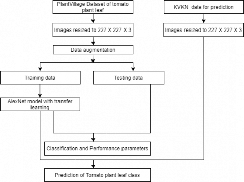
Figure 1. Proposed work flow for classification of Tomato plant leaf
The proposed model of deep learning for the classification of Tomato plant disease is shown in Figure 1. AlexNet, VGG16, GoogLeNet, MobileNetv2, and SqueezeNet are all used to classify the data with the proposed model. This research focuses on the classification of tomato plant disease and validation of models to predict new data from KVKN. The total number of classes for classification is nine, so transfer learning is used in all the cases.
3.1 Healthy and disease tomato plant dataset
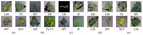
The healthy class of Tomato and eight diseased leaf categories like Tomato BS, EB, LB, LM, MV, SLS, TS, and YLCV are selected from the PlantVillage dataset [29] for the classification objective. The disease class for the tomato plant is selected from the dataset according to their occurrences in the Indian states.
3.2 Dataset augmentation and data resizing
It is necessary to follow the main steps which are common in the analysis [30], one of which is pre-processing, for the smooth operation of any algorithm and to maintain consistency in the analysis. The dataset chosen for the classification purpose is small in size for training a deep learning model. The total images are 900 as there are nine classes, i.e., one healthy and eight diseased ones. When the data is augmented, the dataset size is increased multiple times, and this helps in training the deep network model. In this work, 12 combinations of the augmented dataset are used with the rotation of 90°, 180°, and 270° along with horizontal and vertical flip. Now, after augmentation with the said combination, the size of the dataset is 10800 images.
The images of the dataset need to be resized based on the deep learning model that is going to be used. In the case of AlexNet and SqueezeNet, the required input images should be of size is 227×227×3, whereas, in the case of VGG16, GoogLeNet, and MobileNet, the input image size must be 224×224×3. The input size of the images that are fed to the network must be satisfied for the network to fit the model.
3.3 Creating training and testing dataset
A total dataset is divided into two parts, one of which is used for training the deep learning model, and the other part is used to test the model. In this work, four different combinations of training and testing datasets were used. The combinations are 60-40, 70-30, 80-20, and 90-10, where the first number is the percentage of data from the dataset for training the model, and the second number reveals the testing dataset percentage. For training any of the deep learning models, the following parameters are kept fixed in all the cases. Mini-batch size: states that how many training instances to consider at one time. The learning rate describes the rate at which parameters are updated. The mini-batch size in this work is 10, and the learning rate is 0.0001. The number of iterations over the training set determines the maximum number of epochs.
3.4 Deep learning model
Deep learning models are more advanced versions of basic neural networks. The number of hidden layers is increased in the deep learning model as compared to the traditional neural networks. CNNs consists of the convolution layer, max-pooling layer, ReLU layer, and a classification layer. The combination of these layers decides the design of the model [31]. Deep learning helps in extracting the required features from the input image fed to it [32]. It has the potential of solving complex problems with good accuracy and at a faster rate. The accuracy of the model can be increased by modifying the layers and their combination in the model. The pooling layer reduces the dimensionality of the derived features from the convolution layer [33]. The fully connected layer is a dense network with neuron connections having each node to all node connections. This is connected before the classification layer that classifies the input image into a pre-defined category or class for the prediction of output. As the results are promising for deep learning networks, it has been used widely in many applications [34, 35]. All the models here are implemented with a deep learning toolbox in MATLAB 2019b.
3.4.1 AlexNet
AlexNet is a pre-trained 25 layer deep network that can classify 1000 classes [5]. The aim of this research is to classify the Tomato plant dataset's nine classes into two categories: healthy and diseased. The final three layers of the network are where transfer learning takes place. The flowchart for proposed AlexNet model for classification and prediction of tomato plant disease is shown in Figure 2. The input image dataset is augmented and resized to the size 227x227x3, as the AlexNet requires the input images of this size. AlexNet network model is trained for the four combinations of the training dataset, and the model is tested over the testing dataset. Transfer learning is essential in this model as here; there are nine output classes for classification. The last three layers are replaced with a "fully connected layer" that determines the desired number of outputs to be classified, followed by the “softmax activation function layer”, and finally the “classification output layer” in transfer learning. The testing data is classified with the trained model and performance parameters are evaluated. The tomato plant leaf data from KVKN is resized to 227x227x3 and fed to the trained model for prediction of tomato plant leaf class.
3.4.2 VGG16
VGG 16 is a deeper network than AlexNet, which has a greater number of hidden layers. It has 41 layers in the network [8]. The flowchart for proposed VGG16 model for classification and prediction of tomato plant disease is shown in Figure 3. The input image requirement for this model is 227x227x3. So, the input data of images after augmenting are resized to match this size to fit the model with the required format of input image size. Transfer learning is also performed for VGG16 for the nine classes of Tomato plant leaves. VGG16 model required more time in training the model with the dataset, and this time goes on to increase as the size of training data increases. The testing data is classified with the trained model and performance parameters are evaluated. The tomato plant leaf data from KVKN is resized to 227x227x3 and fed to the trained model for prediction of tomato plant leaf class.
3.4.3 GoogLeNet
LeNet-5, the first convolutional that was developed by LeCun et al. [36], was a seven-level convolutional network. GoogLeNet’s name was given to the winning network of ILSVRC 2014, and this was named after LeNet [6]. This is a 144-layer network, also known as Inception 1. The flowchart for proposed GoogLeNet model for classification and prediction of tomato plant disease is shown in Figure 4. The input size requirement for GoogLeNet is 227x227x3. The input data is augmented and resized to this format and used to train the model. The steps followed in the transfer learning in this network are different than those followed by AlexNet and VGG16. The network was designed with computational competency so that it can be run on separate devices with a limited number of resources. The testing data is classified with the trained model and performance parameters are evaluated. The tomato plant leaf data from KVKN is resized to 227x227x3 and fed to the trained model for prediction of tomato plant leaf class.
Figure 2. Flow chart for classification and prediction of Tomato plant leaf disease using AlexNet
Figure 3. Flow chart for classification and prediction of Tomato plant leaf disease using VGG16
3.4.4 MobileNetv2
MobileNetv2 was developed by a team of researchers from Google. This is an efficient model of MobileNet for mobile and embedded vision applications. This model has convolutions layers that are separable depth-wise, and this helps in reducing the computation by around eight to nine times [37]. The smaller and faster MobileNet is using a width multiplier and resolution, so despite the 154-layer network, the time for training the model is less than the GoogLeNet. The flowchart for proposed MobileNetv2 model for classification and prediction of tomato plant disease is shown in Figure 5. The input size requirement of the model is 224×224×3. The data is augmented and resized to the said format and used to train the model. The testing data is classified with the trained model and performance parameters are evaluated. The tomato plant leaf data from KVKN is resized to 224×224×3 and fed to the trained model for prediction of tomato plant leaf class.
3.4.5 SqueezeNet
SqueezeNet was developed by researchers in 2016 to create a small network that can fit in computer memory [10]. The network is a 68-layer deep learning model and is smaller in size that can train the network in less time as compared to the other networks used in this work. The flowchart for proposed SqueezeNet model for classification and prediction of tomato plant disease is shown in Figure 6. The input size requirement of SqueezeNet is the same as AlexNet i.e., 227 ×227×3. The data is augmented and resized to the said format and used to train the model. The testing data is classified with the trained model and performance parameters are evaluated. The tomato plant leaf data from KVKN is resized to 227×227×3 and fed to the trained model for prediction of tomato plant leaf class.
Figure 4. Flow chart for classification and prediction of Tomato plant leaf disease using GoogLeNet
Figure 5. Flow chart for classification and prediction of Tomato plant leaf disease using MobileNetv2
Figure 6. Flow chart for classification and prediction of Tomato plant leaf disease using SqueezeNet
3.5 Classification and performance parameters
The deep learning model is classified based of model performance and accuracy. The healthy and diseased classes are classified with the five networks and compared based on the accuracy and performance parameters. The performance parameters are evaluated from the confusion matrix of the test dataset. The confusion matrix shows the correct classified classes and the misclassified classes in a certain form. In this, the diagonal elements are the correct classified classes where non-diagonal elements are misclassified, classes. The elements of the confusion matrix are as follows [38].
"$Sensitivity = Recall =\frac{ True \,\,Positive}{True\,\,Positive+False\,\,Negative}$ " (1)
"$Specificity =\frac{ True\,\, Negative }{True\,\, Negative+False\,\, Positive }$ " (2)
"$Precision=\frac{ True\,\, Positive }{True\,\, Positive+False\,\, Positive}$ " (3)
"$Accuracy=\frac{ True\,\, Positive+True\,\, Negative }{True\,\, Positive+True\,\, Negative+ False\,\, Positive+False \,\,Negative}$ " (4)
The number of classes in this work is nine, so the size of the confusion matrix is 9 X 9. With the help of these parameters, each class-wise accuracy of the class for all the used models can be evaluated. Simulation time for training each of the deep learning models with four combinations is noted. The time is measured in seconds.
3.6 Validation of the deep learning models
The above mentioned five models that are trained and tested with the PlantVillage database are further validated with the images captured at KVKN. This helps in predicting the class and its accuracy for each model.
The complete analysis is done on the augmented dataset of 10800 images for nine classes of the Tomato plant from the PlantVillage database. The generated dataset consists of 1200 images for each of the classes. The Tomato plant leaf with a healthy and diseased class is shown in Figure 7 is used in training the model.
Figure 7. Tomato plant leaf images from the training dataset
The training and the testing dataset are a combination of healthy and diseased plant leaves. The data is augmented with a combination of 12 variations is shown in Table 2. In this work, the classification is done by training the model with a different combination of the dataset. The variation of the training-testing dataset is percentage-wise for 60-40, 70-30, 80-20, and 90-10. The number of images in training and testing dataset for the above-mentioned combination is shown in Table 3. For more feature learning, the deep learning models were trained with the augmented dataset and transfer learning is used for the classification of tomato leaf disease with nine classes. This increases the performance of the deep learning model. The VGG16 model takes the lead, with a classification accuracy of 0.9877 for 70% of the training results.
Figure 8. Classified output images for 70% training data using (a) AlexNet, (b) VGG16, (c) GoogLeNet, (d) MobileNetv2, (e) SqueezeNet
Table 2. The Combination is used in augmenting the dataset
|
Original |
90° Rotation |
180° Rotation |
270° Rotation |
|
Horizontal flip |
90° Rotation +Horizontal flip |
180° Rotation +Horizontal flip |
270° Rotation +Horizontal flip |
|
Vertical flip |
90° Rotation +Vertical flip |
180° Rotation +Vertical flip |
270° Rotation +Vertical flip |
Table 3. Training and testing dataset combination used for classification
|
|
Number of images |
|||
|
Training-testing data combinaion |
60-40 |
70-30 |
80-20 |
90-10 |
|
Training data |
6480 |
7560 |
8640 |
9720 |
|
Test data |
4320 |
3240 |
2160 |
1080 |
Table 4. Comparison of proposed work with other existing works
|
Source |
Model |
Accuracy |
|
Rangarajan et al. [3] |
AlexNet |
0.9749 |
|
VGG16 |
0.9729 |
|
|
Wang et al. [11] |
VGG16 |
0.9040 |
|
Hidayatuloh et al. [26] |
SqueezeNet |
0.8692 |
|
Durmus et al. [39] |
AlexNet |
0.9565 |
|
SqueezeNet |
0.9430 |
|
|
Jadhav [40] |
AlexNet |
0.9500 |
|
GoogLeNet |
0.9640 |
|
|
Liu and Wang [41] |
MobileNetv2 |
0.9029 |
|
Proposed model
|
AlexNet |
0.9769 |
|
VGG16 |
0.9877 |
|
|
GoogLeNet |
0.9373 |
|
|
MobileNetv2 |
0.9525 |
|
|
SqueezeNet |
0.9086 |
The hyperparameters of all five networks used here are kept the same for maintaining uniformity. The mini-batch size, maximum epochs, dropout ratio, and the learning rate of 0.0001, is kept in all cases. The classified images using the different models are shown in Figure 8. Herein each of the cases, the training data is 70%, and the classified output is over the remaining 30% of the data. Figure 8(a) depicts the classified output using AlexNet for 30% of the testing data, Figure 8(b) depicts the classified output using VGG16 for 30% of the testing data, Figure 8(c) depicts the classified output using GoogLeNet for 30% of the testing data, Figure 8(d) depicts the classified output using MobileNetv2 for 30% of the testing data, and Figure 8(e) depicts the classified output using SqueezeNet for 30% of the testing data.
Table 4 shows the comparison of the proposed work with other existing works. The performance of the proposed model with 70% of training data is better for AlexNet with 0.9769 as compared to [3, 39, 40]. The accuracy attained by the proposed models of GoogLeNet is 0.9373, MobileNetv2 is 0.9525, SqueezeNet is 0.9086. It is perceived that the VGG16 model is performing supercilious amongst the other models achieving an accuracy of 0.9877.
The accuracy for these networks for each of the combinations of training dataset over testing dataset performance is as shown in Figure 9. It is a general trend that the accuracy goes on increasing as the size of the training data increase. It is seen that the accuracy is decreased for GoogLeNet and SqueezeNet for 70% of the training dataset, but for the other networks, it is increasing. The promising results are seen at 90% of the training dataset. The accuracy for AlexNet is 0.9796, for GoogLeNet, it is 0.9560, and VGG16 is showing the highest accuracy of 0.9917 at 80% training data. The accuracy of 0.9722 for MobileNetv2 is maximum at 90% of the training data. The SqueezeNet model is showing an accuracy of 0.9440 at 80% of the training data.
The amount of time it takes to train the deep learning model is also a significant consideration, as shown in Figure 10. The AlexNet, GoogLeNet, MobileNetv2, and SqueezeNet are having a network training time around the same range except for the VGG16 model that requires very high training time for all the training dataset sizes. It is clear that to achieve the accuracy of 0.9917, at the cost of 49998 seconds for training the model for VGG16. The training time for AlexNet, GoogLeNet MobileNetv2, and SqueezeNet for 80% of the training data is 3792 seconds, 4089 seconds, 10320 seconds, and 1753 seconds respectively. SqueezeNet is a small network, takes less time in training the model for all the training data combinations as compared to other networks.
Figure 9. Accuracy performance of the deep learning networks for different training dataset size
Figure 10. Time for training the deep learning networks for different training dataset size
(a) Confusion matrix for AlexNet using 70% of the training data
(b) Confusion matrix for VGG16 using 70% of the training data
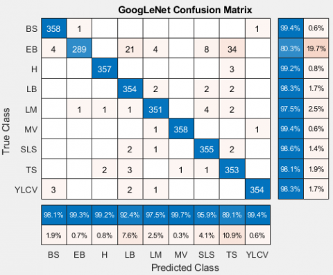
(c) Confusion matrix for GoogLeNet using 70% of the training data
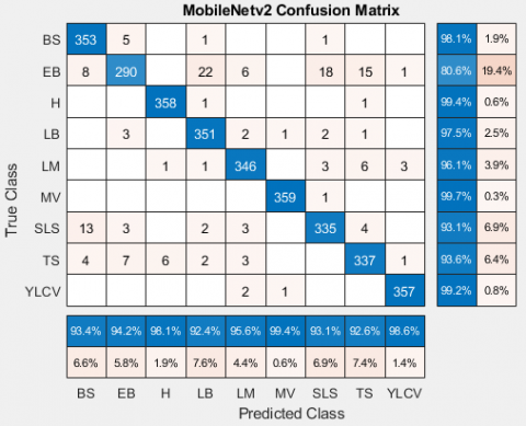
(d) Confusion matrix for MobileNetv2 using 70% of the training data
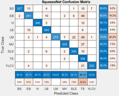
(e) Confusion matrix for SqueezeNet using 70% of the training data
Figure 11. Confusion matrix for deep learning models
The confusion matrix is the matrix that has information about the correct classification and misclassification of each of the classes. Here in this work, there are nine classes for tomato plants consisting of one healthy and other disease classes. Figure 11 shows the confusion matrix for AlexNet, VGG16, GoogLeNet, MobileNetv2, and SqueezeNet for 70% of training data, respectively. The classes in the confusion matrix are BS, EB, H, LB, LM, MV, SLS, TS, and YLCV.
Table 5 shows the performance parameters for each class of the Tomato plant for AlexNet (A), VGG16 (V), GoogLeNet (G), MobileNetv2 (M), and SqueezeNet (S). The performance parameters like sensitivity, specificity, precision, F1 score, and accuracy of each of the classes using all five deep learning models are calculated. The precision is low in all the classes for the SqueezeNet model. The specificity and accuracy of the class for all the model shows good results. Other than Tomato LM and Tomato TS, the F1 Score is also showing superior results for all the classes of tomato. The results are promising for the Tomato MV class for VGG 16 model for all the parameters. Tomato TS shows the least value for the SqueezeNet model for sensitivity. The VGG16 model is overall performing better in classifying and performance parameters.
The five deep learning models after classification are validated with the images captured at KVKN. The validation model helps in understanding how the prediction of the class with the help of a trained model helps classify the unknown images into the particular class with its accuracy.
Table 5. Performance parameters for each of the Tomato plant class
|
Class |
Model |
Sensitivity |
Specificity |
Precision |
F1 score |
Accuracy |
|
BS |
A |
0.9972 |
1 |
1 |
0.9986 |
0.9996 |
|
V |
0.9972 |
0.9989 |
0.9916 |
0.9944 |
0.9987 |
|
|
G |
0.9808 |
0.9993 |
0.9944 |
0.9875 |
0.9972 |
|
|
M |
0.9338 |
0.9975 |
0.9805 |
0.9566 |
0.9901 |
|
|
S |
0.9939 |
0.9886 |
0.9083 |
0.9492 |
0.9891 |
|
|
EB |
A |
0.9333 |
0.9965 |
0.9722 |
0.9523 |
0.9891 |
|
V |
0.9596 |
0.9989 |
0.9916 |
0.9754 |
0.9944 |
|
|
G |
0.9931 |
0.9759 |
0.8027 |
0.8878 |
0.9774 |
|
|
M |
0.9415 |
0.9761 |
0.8055 |
0.8682 |
0.9728 |
|
|
S |
0.9065 |
0.9763 |
0.8083 |
0.8546 |
0.9694 |
|
|
H |
A |
1 |
0.9996 |
0.9972 |
0.9986 |
0.9996 |
|
V |
0.9729 |
1 |
1 |
0.9863 |
0.9969 |
|
|
G |
0.9916 |
0.9989 |
0.9916 |
0.9916 |
0.9981 |
|
|
M |
0.9808 |
0.9993 |
0.9944 |
0.9875 |
0.9972 |
|
|
S |
0.9971 |
0.9951 |
0.9611 |
0.9787 |
0.9953 |
|
|
LB |
A |
1 |
0.9931 |
0.9444 |
0.9714 |
0.9938 |
|
V |
0.9863 |
1 |
1 |
0.9931 |
0.9984 |
|
|
G |
0.9242 |
0.9978 |
0.9833 |
0.9528 |
0.9891 |
|
|
M |
0.9236 |
0.9968 |
0.975 |
0.9486 |
0.9883 |
|
|
S |
0.9222 |
0.9944 |
0.9555 |
0.9386 |
0.9861 |
|
|
LM |
A |
0.952 |
0.9989 |
0.9916 |
0.9714 |
0.9935 |
|
V |
0.9944 |
0.9989 |
0.9916 |
0.993 |
0.9984 |
|
|
G |
0.975 |
0.9968 |
0.975 |
0.975 |
0.9944 |
|
|
M |
0.9558 |
0.9951 |
0.9611 |
0.9584 |
0.9907 |
|
|
S |
1 |
0.9706 |
0.7583 |
0.8625 |
0.9731 |
|
|
MV |
A |
0.9862 |
0.9996 |
0.9972 |
0.9917 |
0.9981 |
|
V |
1 |
1 |
1 |
1 |
1 |
|
|
G |
0.9972 |
0.9993 |
0.9944 |
0.9958 |
0.999 |
|
|
M |
0.9944 |
0.9996 |
0.9972 |
0.9958 |
0.999 |
|
|
S |
0.9624 |
0.9906 |
0.925 |
0.9433 |
0.9876 |
|
|
SLS |
A |
0.952 |
0.9989 |
0.9916 |
0.9714 |
0.9935 |
|
V |
1 |
0.9968 |
0.975 |
0.9873 |
0.9972 |
|
|
G |
0.9594 |
0.9982 |
0.9861 |
0.9726 |
0.9938 |
|
|
M |
0.9305 |
0.9913 |
0.9305 |
0.9305 |
0.9845 |
|
|
S |
0.9214 |
0.993 |
0.9444 |
0.9327 |
0.9848 |
|
|
TS |
A |
0.9818 |
0.9876 |
0.9 |
0.9391 |
0.987 |
|
V |
0.997 |
0.9924 |
0.9388 |
0.967 |
0.9929 |
|
|
G |
0.8914 |
0.9975 |
0.9805 |
0.9338 |
0.9845 |
|
|
M |
0.9258 |
0.992 |
0.9361 |
0.9309 |
0.9845 |
|
|
S |
0.6605 |
0.9992 |
0.9944 |
0.7937 |
0.9425 |
|
|
YLCV |
A |
0.9944 |
0.9996 |
0.9972 |
0.9958 |
0.999 |
|
V |
0.9836 |
1 |
1 |
0.9917 |
0.9981 |
|
|
G |
0.9808 |
0.9993 |
0.9944 |
0.9875 |
0.9972 |
|
|
M |
0.9861 |
0.9989 |
0.9916 |
0.9889 |
0.9975 |
|
|
S |
0.9764 |
0.9903 |
0.9222 |
0.9485 |
0.9888 |
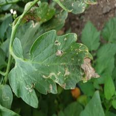
AlexNet: 65% LB
VGG16: 96% LB
GoogLeNet: 95.4% LB
MobileNetV2: 77% BS
SqueezeNet: 100%LB
(b)
AlexNet: 99% EB
VGG16: 97% LB
GoogLeNet: 72.2% LB
MobileNetV2: 58% EB
SqueezeNet: 99%LB
Figure 12. Prediction output of Tomato plant class using AlexNet, VGG16, GoogLeNet, MobileNetv2, and SqueezeNet for the KVKN images
Figure 12 shows the predictions that were attained by the deep learning models. The validation helps in predicting the class of the tomato plant leaf for each of the trained models. The prediction of images is done using the five models that are trained with the PlantVillage database and further validated with KVKN images. It is seen that Figure 12(a) is predicted as LB for all the models except MobileNetV2 predicting it as BS. Figure 12 (b) is predicted as class LB with VGG16, GoogLeNet and SqueezeNet and AlexNet and MobileNetV2 are predicting as EB class. The accuracy of predicting for GoogLeNet, VGG16, and SqueezeNet is promising.
The classification of Tomato Plant leaf images of the PlantVillage database using the deep learning model of AlexNet, VGG16, GoogLeNet, MobileNetv2, and SqueezeNet is done in this work. It is found out that VGG 16 model outperforms with an accuracy of 0.9917 amongst the other models with an accuracy of AlexNet as 0.9796, GoogLeNet as 0.9560, MobileNetv2 as 0.9722, and SqueezeNet as 0.9440 at 80% of training data. In terms of the training time of the model, the maximum time was taken by the VGG16 model at the cost of the highest accuracy achieved. The performance parameters like sensitivity, specificity, precision, F1 score, and accuracy of each of the Tomato plant class with healthy and disease class is calculated and is showing good results throughout affirming the stronger classification process. The model’s classification accuracy and precision provide the information about the performance. The higher these values are, better is the classification. Model can be chosen based on this analysis. The VGG16 model has a higher accuracy and precision for the majority of tomato leaf classes. The validation of these trained models is done on the KVKN images. This classification problem will help in detecting and taking a relevant step for the management of disease and benefits society.
This work is supported by the officials at Krishi Vigyan Kendra Narayangaon, Pune, India for allowing to capture images of tomato plant in the field.
[1] Arivazhagan, S., Shebiah, R.N., Ananthi, S., Varthini, S.V. (2013). Detection of unhealthy region of plant leaves and classification of plant leaf diseases using texture features. Agricultural Engineering International: CIGR Journal, 15(1): 211-217.
[2] Al Bashish, D., Braik, M., Bani-Ahmad, S. (2010). A framework for detection and classification of plant leaf and stem diseases. 2010 international conference on signal and image processing, Chennai, India, pp. 113-118. https://doi.org/10.1109/ICSIP.2010.5697452
[3] Rangarajan, A.K., Purushothaman, R., Ramesh, A. (2018). Tomato crop disease classification using pre-trained deep learning algorithm. Procedia Computer Science, 133: 1040-1047. https://doi.org/10.1016/j.procs.2018.07.070
[4] Singh, V., Misra, A.K. (2017). Detection of plant leaf diseases using image segmentation and soft computing techniques. Information Processing in Agriculture, 4(1): 41-49. https://doi.org/10.1016/j.inpa.2016.10.005
[5] Krizhevsky, A., Sutskever, I., Hinton, G.E. (2012). Imagenet classification with deep convolutional neural networks. Advances in Neural Information Processing Systems, 25: 1097-1105.
[6] Szegedy, C., Liu, W., Jia, Y., Sermanet, P., Reed, S., Anguelov, D., Rabinovich, A. (2015). Going deeper with convolutions. Proceedings of the IEEE Conference on Computer Vision and Pattern Recognition, Boston, MA, USA, pp. 1-9. https://doi.org/10.1109/CVPR.2015.7298594
[7] He, K., Zhang, X., Ren, S., Sun, J. (2016). Deep residual learning for image recognition. In Proceedings of the IEEE Conference on Computer Vision and Pattern Recognition, Las Vegas, NV, USA, pp. 770-778. https://doi.org/10.1109/CVPR.2016.90
[8] Simonyan, K., Zisserman, A. (2014). Very deep convolutional networks for large-scale image recognition. arXiv preprint arXiv:1409.1556.
[9] Huang, G., Liu, Z., Van Der Maaten, L., Weinberger, K.Q. (2017). Densely connected convolutional networks. Proceedings of the IEEE Conference on Computer Vision and Pattern Recognition, Honolulu, HI, USA, pp. 4700-4708. https://doi.org/10.1109/CVPR.2017.243
[10] Iandola, F.N., Han, S., Moskewicz, M.W., Ashraf, K., Dally, W.J., Keutzer, K. (2016). SqueezeNet: AlexNet-level accuracy with 50x fewer parameters and< 0.5 MB model size. arXiv preprint arXiv:1602.07360.
[11] Wang, G., Sun, Y., Wang, J. (2017). Automatic image-based plant disease severity estimation using deep learning. Computational Intelligence and Neuroscience. https://doi.org/10.1155/2017/2917536
[12] Lu, Y., Yi, S., Zeng, N., Liu, Y., Zhang, Y. (2017). Identification of rice diseases using deep convolutional neural networks. Neurocomputing, 267: 378-384. https://doi.org/10.1016/j.neucom.2017.06.023
[13] Jeon, W.S., Rhee, S.Y. (2017). Plant leaf recognition using a convolution neural network. International Journal of Fuzzy Logic and Intelligent Systems, 17(1): 26-34. http://dx.doi.org/10.5391/IJFIS.2017.17.1.26
[14] Han, X., Zhong, Y., Cao, L., Zhang, L. (2017). Pre-trained AlexNet architecture with pyramid pooling and supervision for high spatial resolution remote sensing image scene classification. Remote Sensing, 9(8): 848. https://doi.org/10.3390/rs9080848
[15] Zhao, G., Liu, F., Oler, J.A., Meyerand, M.E., Kalin, N.H., Birn, R.M. (2018). Bayesian convolutional neural network based MRI brain extraction on nonhuman primates. Neuroimage, 175: 32-44. https://doi.org/10.1016/j.neuroimage.2018.03.065
[16] Wiesner-Hanks, T., Stewart, E.L., Kaczmar, N., DeChant, C., Wu, H., Nelson, R.J., Gore, M.A. (2018). Image set for deep learning: Field images of maize annotated with disease symptoms. BMC Research Notes, 11(1): 1-3. https://doi.org/10.1186/s13104-018-3548-6
[17] Toğaçar, M., Cömert, Z., Ergen, B. (2020). Classification of brain MRI using hyper column technique with convolutional neural network and feature selection method. Expert Systems with Applications, 149: 113274. https://doi.org/10.1016/j.eswa.2020.113274
[18] Lenz, B., Hasselbruch, H., Mehner, A. (2020). Automated evaluation of Rockwell adhesion tests for PVD coatings using convolutional neural networks. Surface and Coatings Technology, 385: 125365. https://doi.org/10.1016/j.surfcoat.2020.125365
[19] Rehman, A., Naz, S., Razzak, M.I., Akram, F., Imran, M. (2020). A deep learning-based framework for automatic brain tumors classification using transfer learning. Circuits, Systems, and Signal Processing, 39(2): 757-775. https://doi.org/10.1007/s00034-019-01246-3
[20] Pereira, C.S., Morais, R., Reis, M.J.C.S. (2019). Deep learning techniques for grape plant species identification in natural images. Sensors (Switzerland), 19(22): 4850. https://doi.org/10.3390/s19224850
[21] Türkoğlu, M., Hanbay, D. (2019). Plant disease and pest detection using deep learning-based features. Turkish Journal of Electrical Engineering & Computer Sciences, 27(3): 1636-1651. https://doi.org/10.3906/elk-1809-181
[22] Liu, B., Zhang, Y., He, D., Li, Y. (2018). Identification of apple leaf diseases based on deep convolutional neural networks. Symmetry, 10(1): 11. https://doi.org/10.3390/sym10010011
[23] Lu, X., Wu, H., Zeng, Y. (2019). Classification of Alzheimer’s disease in MobileNet. Journal of Physics: Conference Series, 1345(4): 042012. https://doi.org/10.1088/1742-6596/1345/4/042012
[24] Kamal, K.C., Yin, Z., Wu, M., Wu, Z. (2019). Depthwise separable convolution architectures for plant disease classification. Computers and Electronics in Agriculture, 165: 104948. https://doi.org/10.1016/j.compag.2019.104948
[25] Başaran, E., Cömert, Z., Çelik, Y. (2020). Convolutional neural network approach for automatic tympanic membrane detection and classification. Biomedical Signal Processing and Control, 56: 101734. https://doi.org/10.1016/j.bspc.2019.101734
[26] Hidayatuloh, A., Nursalman, M., Nugraha, E. (2018). Identification of tomato plant diseases by Leaf image using squeezenet model. In 2018 International Conference on Information Technology Systems and Innovation (ICITSI), Bandung, Indonesia, pp. 199-204. https://doi.org/10.1109/ICITSI.2018.8696087
[27] Khamparia, A., Gupta, D., de Albuquerque, V.H.C., Sangaiah, A.K., Jhaveri, R.H. (2020). Internet of health things-driven deep learning system for detection and classification of cervical cells using transfer learning. The Journal of Supercomputing, 76: 8590-8608. https://doi.org/10.1007/s11227-020-03159-4
[28] Ayu, H.R., Surtono, A., Apriyanto, D.K. (2021). Deep learning for detection cassava leaf disease. In Journal of Physics: Conference Series, 1751(1): 012072. https://doi.org/10.1088/1742-6596/1751/1/012072
[29] Mohanty, S.P., Hughes, D.P., Salathé, M. (2016). Using deep learning for image-based plant disease detection. Frontiers in Plant Science, 7: 1419. https://doi.org/10.3389/fpls.2016.01419
[30] Dyrmann, M., Karstoft, H., Midtiby, H.S. (2016). Plant species classification using deep convolutional neural network. Biosystems Engineering, 151: 72-80. https://doi.org/10.1016/j.biosystemseng.2016.08.024
[31] Gers, F.A., Schmidhuber, J., Cummins, F. (2000). Learning to forget: Continual prediction with LSTM. Neural Computation, 12(10): 2451-2471. https://doi.org/10.1162/089976600300015015
[32] LeCun, Y., Bengio, Y., Hinton, G. (2015). Deep learning. Nature, 521(7553): 436-444. https://doi.org/10.1038/nature14539
[33] Kamilaris, A., Prenafeta-Boldú, F.X. (2018). Deep learning in agriculture: A survey. Computers and Electronics in Agriculture, 147: 70-90. https://doi.org/10.1016/j.compag.2018.02.016
[34] Ding, J., Chen, B., Liu, H., Huang, M. (2016). Convolutional neural network with data augmentation for SAR target recognition. IEEE Geoscience and Remote Sensing Letters, 13(3): 364-368. https://doi.org/10.1109/LGRS.2015.2513754
[35] Volpi, M., Tuia, D. (2016). Dense semantic labeling of subdecimeter resolution images with convolutional neural networks. IEEE Transactions on Geoscience and Remote Sensing, 55(2): 881-893. https://doi.org/10.1109/TGRS.2016.2616585
[36] LeCun, Y., Bottou, L., Bengio, Y., Haffner, P. (1998). Gradient-based learning applied to document recognition. Proceedings of the IEEE, 86(11): 2278-2324. https://doi.org/10.1109/5.726791
[37] Sandler, M., Howard, A., Zhu, M., Zhmoginov, A., Chen, L.C. (2018). MobileNetV2: Inverted residuals and linear bottlenecks. 2018 IEEE/CVF Conference on Computer Vision and Pattern Recognition, Salt Lake City, UT, USA, pp. 4510-4520. https://doi.org/10.1109/CVPR.2018.00474
[38] Sathyanarayana, A., Joty, S., Fernandez-Luque, L., Ofli, F., Srivastava, J., Elmagarmid, A., Taheri, S. (2016). Sleep quality prediction from wearable data using deep learning. JMIR mHealth and uHealth, 4(4): e125. https://doi.org/10.2196/mhealth.6562
[39] Durmuş, H., Güneş, E.O., Kırcı, M. (2017). Disease detection on the leaves of the tomato plants by using deep learning. 2017 6th International Conference on Agro-Geoinformatics, Fairfax, VA, USA, pp. 1-5. https://doi.org/10.1109/Agro-Geoinformatics.2017.8047016
[40] Jadhav, S.B. (2019). Convolutional neural networks for leaf image-based plant disease classification. IAES International Journal of Artificial Intelligence, 8(4): 328. https://doi.org/10.11591/ijai.v8.i4.pp328-341
[41] Liu, J., Wang, X. (2020). Early recognition of tomato gray leaf spot disease based on MobileNetv2-YOLOv3 model. Plant Methods, 16: 83. https://doi.org/10.1186/s13007-020-00624-2