Vasileios Papageorgiou
© 2021 IIETA. This article is published by IIETA and is licensed under the CC BY 4.0 license (http://creativecommons.org/licenses/by/4.0/).
OPEN ACCESS
Brain tumor detection or brain tumor classification is one of the most challenging problems in modern medicine, where patients suffering from benign or malignant brain tumors are usually characterized by low life expectancy making the necessity of a punctual and accurate diagnosis mandatory. However, even today, this kind of diagnosis is based on manual classification of magnetic resonance imaging (MRI), culminating in inaccurate conclusions especially when they derive from inexperienced doctors. Hence, trusted, automatic classification schemes are essential for the reduction of humans’ death rate due to this major chronic disease. In this article, we propose an automatic classification tool, using a computationally economic convolutional neural network (CNN), for the purposes of a binary problem concerning MRI images depicting the existence or the absence of brain tumors. The proposed model is based on a dataset containing real MRI images of both classes with nearly perfect validation-testing accuracy and low computational complexity, resulting a very fast and reliable training-validation process. During our analysis we compare the diagnostic capacity of three alternative loss functions, validating the appropriateness of cross entropy function, while underlining the capability of an alternative loss function named Jensen-Shannon divergence since our model accomplished nearly excellent testing accuracy, as with cross-entropy. The multiple validation tests applied, enhancing the robustness of the produced results, render this low-complexity CNN structure as an ideal and trustworthy medical aid for the classification of small datasets.
artificial intelligence, brain MRI, convolutional neural networks, cross-entropy, Jensen-Shannon divergence, loss functions, tumor detection
Brain tumor, known as intracranial tumor, is an abnormal mass of tissue in which cells grow unnaturally and uncontrollably. Brain tumors make up less than 2% of human cancer, according to World Health Organization, although its severe morbidity and compilations, render early diagnosis a very important concept in modern medicine [1]. Brain tumors can be deadly, affecting significantly a patient’s life without discriminating between men, women or children. Furthermore, according to national brain tumor society, over 700.000 citizens in the United States are living with a primary brain tumor, while it was predicted that over 87.000 citizens would be diagnosed with a brain tumor in 2020 [2].
The existing tumors are categorized into four grades; grade I represents the safest form of brain tumors, including only benign tumors that are curable via surgery, slow-growing with patients having a long-term survival rate. Some significant examples of grade I tumors are pilocytic astrocytoma, craniopharyngioma, gangliocytoma and ganglioglioma. The second category is grade II tumors, which are characterized by relatively slow growing rate and may recur after a brain surgery.
On the other hand, grade III and grade IV are high-grade tumors that are deemed as malignant. Another significant characteristic of these tumors is that they cannot be cured via surgery usually because of their high recurrence probability. Grade III tumors tend to recur in the future; some examples are anaplastic astrocytoma, anaplastic ependymoma and anaplastic oligodendeoglioma. Grade IV tumors represent an irreversible situation due to their probable transition to neighboring tissues, reducing patient’s life expectancy significantly. Signature instances are pineoblastoma, medulloblastoma, ependymoblastoma and glioblastoma multiforme (GBM) [3].
The most frequently observed benign tumors are meningiomas, pituitary adenomas and schwannomas while the category of malignant tumors includes the various cases of gliomas representing the 78% of all malignant brain tumors. Meningiomas are the most common benign intracranial tumors comprising 10 to 15% of all neoplasms. Pituitary adenomas are the most common intracranial tumors after meningiomas, gliomas and schwannomas, affecting patients often in their 30s and 40s, while schwanommas arise along nerves, comprised of cells that normally provide the electrical insulation for the nerve cell. Gliomas arise from the supporting cells of brain called glia, including ependynomas, medulloblastomas, astrocytomas and GBM which is the most invasive type of glial tumor [4].
MRI images are the most efficient medical tools for manual tumor diagnosis, where experienced doctors are usually not just able to diagnose a tumor’s existence but can decide if the examined tumor is malignant. Primarily, MRI images depicting brain tumors, contain smaller or wider regions inside the cerebrum’s area of slightly lighter colors. In cases, where accurate diagnosis of brain tumors is necessary, experts utilize MRI images with contrast, where a dye is given to the patient intravenously prior to the scan. Machine and Deep Learning are the domains of statistical methods and algorithms that can be used to solve the complex issue of efficient brain tumor diagnosis based on MRI images.
There is a variety of algorithms that have widely emerged in the field of medical imaging as a part of artificial intelligence, while their main goal is to learn inherent patterns of training data using algorithms like Artificial Neural Networks (ANN) [5], K-Nearest Neighbors (KNN) [6] and Support Vector Machine (SVM) [7, 8]. However, another category of algorithms named Convolutional Neural Networks (CNN) seem to be the most ideal way of dealing with image or video problems due to higher classification performances.
There is a variety of papers dealing with binary and multiclass brain tumor diagnosis problems using a series of state-of-the-art deep convolutional neural networks. Many articles initiate their analysis with image prepossessing, image augmentation or segmentation procedures to enhance their algorithm’s classification capability. The most relevant category of articles compared to our analysis are articles dealing with binary classification of benign and malignant tumors. Babu et al. [9], Seetha and Raja [10], Kulkarni and Sundari [11] and Pathak et al. [12], combine preprocessing and image augmentation techniques with CNNs to classify benign and malignant brain tumors with accuracies 94.1%, 97.5%, 98% and 98% respectively. More precisely, Kulkarni and Sundari [11] utilize AlexNet, a well-known deep convolutional neural network for the purposes of this classification case. A CNN-SVM architecture is proposed for binary classification with corresponding accuracies 88.54%, 95% and 95.62% [13-15]. In the first part of the architecture, a CNN is responsible for the efficient extraction of features according to which an SVM classifies the images. Sert et al. [14] and Ӧzyurt et al. [15], suggest ResNet for the first part of the CNN-SVM architecture, while the images were preprocessed using resolution enhancement and entropy segmentation techniques. Simultaneously, Ӧzyurt et al. [15] compare their model with a CNN-KNN on the same dataset with an accuracy of 90.62%. An ELM-LRF structure is proposed by Ari and Hanbay [16] with 97.1% accuracy; basic CNN structures are used for the classification of the MRI images with 97.87% and 91.82% accuracy [5, 17]. These papers’ analysis is based on segments of MRI images containing only the tumor region. Similar methodology is followed by Banerjee [18] with the difference that the utilized model is based on transfer learning with an accuracy of 97.19%. Another binary approach between low-grade gliomas (LGG) and GBM is displayed in the studies [18, 19], based on histopathology images classified by a CNN-SVM hybrid with an accuracy of 97.8%. Murali and Meena [20] display another instance of binary classification by categorizing MRI images containing gliomas and meningiomas, accomplishing 97.2% accuracy. Finally, the researchers [21, 22], are of particular interest because the authors use one of the datasets that we utilize for the training-validation of their CNNs. Both papers propose preprocessing and augmentation of their dataset with maximum accuracies of 95%. The 95% accuracy of Ref. [23] achieved by one of the three proposed CNNs, is based on ResNet50 architecture; although with obvious overfitting problems, as Saxena et al. state. Another successful attempt of classifying images with and without brain tumors is displayed by Sajja and Kalluri [24], where the usage of a CNN on a BRATS dataset containing 577 images, gives an accuracy of 96.15%, tested on 182 images.
As we mentioned above, there are analyses dealing with multiclass classification problems using a variety of preprocessing techniques and CNNs. Das et al. [25], Afshar et al. [26] and Alqudah et al. [27] propose CNN structures to classify images representing three kinds of brain tumors; meningiomas, pituitary adenomas and gliomas of a public dataset with accuracies 94.39%, 90.89% and 98%, comparing classification performance on cropped, uncropped and segmented images. Mittal and Kumar [28] classify MRI images concerning three tumor categories plus a class for the negative diagnoses with the aid of an AiCNN, mixing five different models to 1 and accomplishing a testing accuracy of 98.8%. Simultaneously, Mohsen et al. [29] and Sajjad et al. [30], achieve a classification rate of 93.94% and 94.58% respectively, on images that were previously segmented.
On the other hand, a DenseNet-LSTM hybrid is utilized for a four class tumor classification problem reaching 92.13% on a public database [31], while Sultan et al. [32] validate their CNN model on two databases containing three classes of tumors (meningiomas, pituitary adenomas and gliomas) and (Grade II, Grade III, Grade IV) with overall accuracies of 96.13% and 98.7%. Another approach is the usage of pre-trained CNNs [33], with an accuracy of 97.64% and 98% accomplished on two datasets consisting of three and four tumor classes respectively. Finally, Zhao and Jia [34] takes advantage of a deep convolutional neural network to segment the image parts containing the tumor and classify these parts into five categories with an accuracy of 81%.
This section illustrates the proposed methodology used for the binary classification. Our methodology consists of four basic stages; image preprocessing and augmentation, construction and tuning of the CNN, evaluation based on performance measures and comparisons between various loss functions.
3.1 Preprocessing
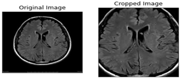
Our dataset consists of two classes of MRI images depicting images with and without tumor, while their original size varies among them. We generated new MRI instances via image augmentation by slightly changing the basic properties of the initial images, like brightness, angle, orientation and zoom. This technique is often used in related work because these new images represent other possible cases of patients’ MRI and simultaneously enhance the robustness of neural networks [35]. Another element that makes this technique so popular is the fact that especially in medical problems, datasets are small resulting in unreliable models. The second step is to crop the black parts around the cranium of each MRI image, which contain no valuable information for the classification (shown in Figure 1). As a result, we keep the important part of the image that is the part of the brain where the tumor takes place. This technique not only makes the process more accurate, but also shortens the period needed for the training of the CNN. Another advantage of the aforementioned procedure, is that by cropping the space around the brain we avoid unwanted correlations between the two classes according to the position of the brain inside the MRI image.
a) Existence of Tumor
b) Absence of Tumor
Figure 1. Original and cropped images representing brain MRI images with and without tumor
3.2 Convolutional neural networks
CNNs are a category of neural networks that is focused on image or video related problems, usually taking an order 3 tensor as their input. For instance, a colored image with M rows, N columns and 3 channels (in the RGB system) is an order 3 tensor, denoted as $\boldsymbol{X}^{1} \in \mathbb{R}^{M \times N \times 3}$ Although, there are occasions where we work with tensors of lower or higher order, e.g. when our images are black and white, they represent tensors of order 2. A CNN consists of a series of successive layers; convolutional, pooling, batch normalization, fully connected layers and a loss layer. These layers constitute the two main parts of a CNN, which are the parts of feature extraction and feature selection [36].
3.2.1 Forward run and backward propagation
Let $\boldsymbol{X}^{k}$ be the input of the k–th layer of a CNN and $\boldsymbol{w}^{k}$ be the set of trainable parameters of each layer. Our input $\boldsymbol{X}^{1}$ passes through a series of layers until the last layer – the loss layer – where with the contribution of the loss function, we combine the output $\mathrm{y}_{j}$, and the label of the $j$–th image $\hat{y}_{j}$ to produce an error $\boldsymbol{Z}$. This process is called forward run and takes place during the training phase. During the training process there is a second procedure called backward propagation. This procedure utilizes the produced error, to modify all trainable parameters of the CNN according to a learning algorithm, e.g. stochastic gradient decent
$\left(w^{k}\right)^{i+1}=\left(w^{k}\right)^{i}-\eta \frac{\partial z}{\partial\left(w^{k}\right)^{i}}$, (1)
where, $\eta$ denotes the learning rate of the algorithm and i the training’s i-th iteration [37]. Learning rate η represents a hyperparameter that its misplaced selection may lead to non-optimum results.
3.2.2 Convolutional layer
The most signature layer of a CNN, belonging to its first part of feature extraction. Convolution is a local operation which role is the extraction of various patterns from the input images resulting in an efficient classification. Convolutional layers are consisted of multiple convolutional kernels which are the layers’ trainable parameters, modified during each iteration. Let $X^{k} \in \mathbb{R}^{M^{k} \times N^{k} \times D^{k}}$ be the input of the k–th convolutional layer and $\mathbf{F} \in \mathbb{R}^{m \times n \times d^{k} \times s}$ be an order four tensor representing the s kernels of k–th layer, of spatial span $m \times n$. The output of the k–th convolutional layer will be an order three tensor denoted as $\left.\boldsymbol{X}^{k+1}\right) \in \mathbb{R}^{M^{k}-m+1 \times N^{k}-n+1 \times S}$ which elements result from
$y_{i} k_{, j} k_{s}=\sum_{i=0}^{m} \sum_{j=0}^{n} \sum_{l=0}^{d^{k}} F_{i, j, d^{k}, s} \times x_{i^{k}, j^{k}, l}^{k}$ (2)
Eq. (2) is repeated for all $0 \leq s \leq S$ and for any spatial location satisfying $0 \leq i^{k} \leq M^{k}-m+1$ and $0 \leq j^{k} \leq N^{k}-n+1$. CNNs usually combine successive convolutional layers aiming to detect larger spatial patterns of the input images [37, 38]. The utilization of convolutional layers is often accompanied by the operation of zero padding that maintains the image’s dimension unchanged during the process.
3.2.3 Pooling layer
Let $\boldsymbol{X}^{k} \in \mathbb{R}^{M^{k} \times N^{k} \times D^{k}}$ be the input of the $k$–th layer that is now a pooling layer with a spatial span of $m \times n$. These layers are parameter free, which means that there are no parameters to be trained. We assume that$m$ divides $M$ and $n$ divides $N$ and the stride equals the pooling spatial span. The output is an order three tensor denoted as $\boldsymbol{Y}^{k} \in \mathbb{R}^{M^{k+1} \times N^{k+1} \times D^{k+1}}$, where
$M^{k+1}=\frac{M^{k}}{m}, N^{k+1}=\frac{N^{k}}{n}, D^{k+1}=D^{k}$, (3)
while the polling layer operates upon $\boldsymbol{X}^{k}$ channel by channel independently. There is a variety of pooling operations with max pooling and average pooling being widely used. In our analysis, we used max pooling, culminating in outputs produced according to formula
$y_{i^{k}, j^{k}, d}=\max _{0 \leq i \leq m, 0 \leq j \leq n} x_{i^{k} \times m+i, j^{k} \times n+j, d}^{k}$ (4)
where, $0 \leq i^{k} \leq M^{k}, 0 \leq j^{k} \leq N^{k}$ and $0 \leq d \leq D^{k}$.
Intuitively, pooling layers are used to decrease the dimensions of the output tensors whereas maintaining the most crucial detected patterns [39].
3.2.4 Fully connected layer
This layer belongs to the second part of a CNN and its role is the effective selection of features extracted by the first part. The input of the first fully connected layer is a high dimensional vector containing all extracted features produced by a flattening operation. After the last fully connected layer, there is always a classification function, e.g. sigmoid, softmax, tanh etc. producing a real value $y_{j}$ that will be compared with the expected value (label) $\hat{y}_{i}$ based on the selected loss function. In our occasion, we deem that the utilization of the sigmoid function
$\hat{y}_{j}=\frac{e^{x_{j}}}{1+e^{x_{j}}}, \quad x_{j} \in \mathbb{R}$ (5)
would be appropriate for this binary problem. Intuitively, $y_{j} \in(0,1)$ represents the probability that the input image depicts a tumor’s existence.
Dropout is another important concept, which is a technique used to improve the generalization of the learning method, minimizing the probability of overfitting. It sets the parameters connected to a certain percentage of nodes in the network to zero [40]. Finally, important transition mediums connecting the aforementioned layers are the operations of ReLU and batch normalization. The ReLU function is defined as
$y_{i, j, d}=\max \left(0, x_{i, j, d}^{k}\right)$ (6)
with $0 \leq i \leq M^{k}, 0 \leq j \leq N^{k}$ and $0 \leq d \leq D^{k}$, aiming to transfer only the purposive elements for the classification, while batch normalization makes neural networks faster and stabler by normalizing the layer’s input through re-scaling and re-centering during each iteration. The exact reasons why batch normalization increases a network’s accuracy are under discussion [41].
3.3 Loss functions
As we previously mentioned, a selected loss function takes $\boldsymbol{y}_{j}$ and $\widehat{\boldsymbol{y}}_{j}$ as inputs and produces an error z, according to which, the back-propagation process takes place. In this paper, we will compare the performance of four loss functions which are cross-entropy, hinge, squared hinge and Jensen-Shannon divergence.
Cross-entropy:
$S_{\text {cross }}\left(\boldsymbol{y}_{j}, \widehat{\boldsymbol{y}}_{j}\right)=-\frac{1}{n} \sum_{k=1}^{n} y_{j k} \log \hat{y}_{j k}$ (7)
This loss function measures the expected inaccuracy of events observed with distribution $\widehat{\boldsymbol{y}}_{j}$ while the information contained in the events is valuated according to $\boldsymbol{y}_{i}$. The mentioned $\widehat{\boldsymbol{y}}_{j}$ and $\boldsymbol{y}_{i}$ are vectors containing n instances of classified images included in the training-testing process.
Hinge:
$H\left(\boldsymbol{y}_{j}, \widehat{\boldsymbol{y}}_{j}\right)=\frac{1}{n} \sum_{k=1}^{n} \max \left(0,1-y_{j k} \hat{y}_{j k}\right)$. (8)
Squared Hinge:
$S q H\left(\boldsymbol{y}_{j}, \widehat{\boldsymbol{y}}_{j}\right)=\frac{1}{n} \sum_{k=1}^{n} \max \left(0,1-y_{j k} \hat{y}_{j k}\right)^{2}$. (9)
Hinge and squared hinge functions are frequently used in machine learning algorithms and more precisely in SVM models.
Jensen-Shannon divergence:
$\operatorname{JSD}\left(\boldsymbol{y}_{j}, \hat{\boldsymbol{y}}_{j}\right)=\frac{1}{2}\left(K L\left(\boldsymbol{y}_{j}, \frac{\boldsymbol{y}_{j}+\hat{\boldsymbol{y}}_{j}}{2}\right)+K L\left(\hat{y}_{j}, \frac{\boldsymbol{y}_{j}+\hat{\boldsymbol{y}}_{j}}{2}\right)\right)$, (10)
where, n is the number of samples and KL is the notation for Kullback-Leibler divergence
$K L\left(\boldsymbol{y}_{j}, \widehat{\boldsymbol{y}}_{j}\right)=\frac{1}{n} \sum_{k=1}^{n} y_{j k} \log \frac{y_{j k}}{\hat{y}_{j k}}$. (11)
3.4 Classification measures
After the completion of the training phase, we test the performance of our model using a series of validation measures. We will invoke four well-known measures named accuracy, sensitivity, specificity and F1 score which can be defined as
Accuracy $=\frac{T P+T N}{T P+T N+F P+F N}$ (12)
Sensitivity $=\frac{T P}{T P+F N}$ (13)
Specificity $=\frac{T F}{T F+F P}$ (14)
$F 1$ score $=\frac{2 T P}{2 T P+F P+F N}$. (15)
Sensitivity represents the probability that the CNN correctly diagnoses the presence of a tumor in an MRI image. On the other hand, specificity represents the probability that the CNN correctly diagnoses the absence of a tumor while F1 score is the harmonic mean of precision and sensitivity.
4.1 Dataset
For the purposes of our analysis, we combine two public databases named Brain MRI Images for Brain Tumor Detection and Br35H::Brain Tumor Detection 2020, published in Kaggle. The first dataset contains 253 MRI images, from which 98 represent cases of healthy brain MRI and the remaining 155 represent the existence of tumors, while the second one contains 1500 images for each category of the binary classification problem, producing a nearly balanced combined dataset of 3253 instances. After the application of augmentation, the final dataset includes 16.265 MRI images, providing 13.012, 2.440 and 813 images for training, validation and testing respectively.
4.2 CNN architecture
We propose a low complexity CNN architecture composed of seven primary layers as shown in Figure 2. Four of them (two convolutional and two max pooling) are responsible for feature extraction while the remaining three layers (fully connected) utilize these features to accomplish a high diagnostic efficiency. The inputs of our CNN are two-dimensional matrices representing the gray-scale MRI images of size 120x120. We concluded to this selection after experimentation, because the chosen relatively small input size, implies lower computational cost without deteriorating our model’s accuracy.
Figure 2. The proposed low-complexity CNN structure for MRI images classification, consisting of 7 trainable layers
Figure 3. Training, validation loss and accuracy during 75 epochs using cross-entropy loss function
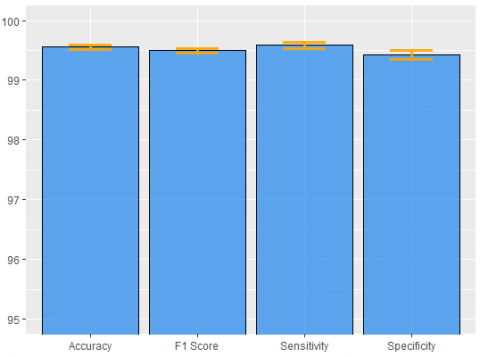
Figure 4. Mean performance measures of validation process ± standard deviations for cross entropy, revealing a slightly higher sensitivity
The input matrices are transmitted to the first convolutional layer containing 32 kernels of size 9x9, while the feature maps extracted from this layer pass through a max pooling layer of spatial span 4x4, retaining only the max values of the 4x4 feature maps’ subregions. This structure is repeated once more containing a 5x5 convolutional and a 4x4 max pooling layer. We used same padding before the application of the convolutional operation. Each of these layers is followed by batch normalization and ReLU operations.
The second part is consisted of three fully connected layers containing 2048, 256 and 1 node respectively. Between the first two fully connected layers, there is a dropout layer eliminating overfitting effects. We trained our model for 75 epochs based on Adam optimizer with $\eta=0.001$, which seems to have a more unstable but more effective training process compared to stochastic gradient descent, as we observe based on Figure 3.
According to the proposed structure, we reach perfect training accuracy while in Figure 4 we observe a validation accuracy of 99.56%, sensitivity of 99.59%, specificity of 99.43% and f1 score of 99.50%. These results are the mean values produced by executing the whole training – validation process multiple times with different sampling combinations for training and validation, aiming to increase the reliability of our method. The corresponding standard deviations of the aforementioned results are 0.11, 0.256, 0.171 and 0.144. Applying the trained model to the test set we achieve similar, almost excellent detection capacity. The slightly higher sensitivity witnesses that our model yields just a bit better results on images displaying tumors. Our training-validation on 13.012 and 2.440 images lasted only for 2.123 seconds, which is translated in 28.3 seconds per epoch, running on a GPU and more specifically on a NVIDIA GeForce GTX 760 graphics card. The existence of a more recently released GPU would produce an even shorter training-validation process.
4.3 Performance comparison of loss functions
In this section, we examine the results of the diagnostic procedure of four loss functions; cross-entropy, hinge loss, square hinge loss and Jensen Shannon divergence (JSD). For this attempt, we utilize the CNN structure that we extensively present above. The only remarkable difference is that during the training of our CNN with hinge and squared hinge loss, we label the absence of tumor with -1 and the existence with 1, while we substitute sigmoid with hyperbolic tangent function (tanh). Another important note is the necessary change of learning rate, where we employed $\eta=0.0001$ for $\mathrm{JSD}$ and $\eta=0.00001$ for the two remaining loss functions.
Table 1. Performance measures for the validation process of the selected loss functions, proposing the utilization of cross – entropy
|
Loss function |
Accuracy |
Sensitivity |
Specificity |
F1 score |
|
Cross-Entropy |
99.56% |
99.59% |
99.43% |
99.50% |
|
Hinge |
98.72% |
98.90% |
98.58% |
98.70% |
|
Squared Hinge |
98.97% |
98.99% |
98.99% |
98.95% |
|
JSD |
99.38% |
99.31% |
99.42% |
99.34% |
Table 2. Performance measures for the testing process of the selected loss functions, highlighting the selection of cross-entropy for brain tumor detection.
|
Loss function |
Accuracy |
Sensitivity |
Specificity |
F1 score |
|
Cross-Entropy |
99.62% |
99.48% |
99.56% |
99.49% |
|
Hinge |
98.73% |
98.87% |
98.56% |
98.69% |
|
Squared Hinge |
98.53% |
98.27% |
98.85% |
98.56% |
|
JSD |
99.33% |
99.25% |
99.20% |
99.24% |
Table 3. Presentation of binary classification methods’ performances, displayed in related work
|
|
Model |
Best Testing Accuracy |
Classification Method |
|
1 |
Manjunath et al. [5] |
97.87% |
CNN |
|
2 |
Babu et al. [9] |
94.10% |
CNN |
|
3 |
Seetha and Raja [10] |
97.50% |
CNN |
|
4 |
Kulkarni and Sundari [11] |
98.33% |
CNN |
|
5 |
Pathak et al. [12] |
98.00% |
CNN |
|
6 |
Ari and Hanbay [16] |
97.18% |
ELM-LRF |
|
7 |
Hossain et al. [17] |
91.82% |
CNN |
|
8 |
Banerjee et al. [18] |
97.19% |
CNN-Transfer Learning |
|
9 |
Xu et al. [19] |
97.80% |
CNN (Histop. images) |
|
10 |
Mohammed [20] |
95.00% |
CNN (same dataset) |
|
11 |
Saxena [21] |
95.00% |
CNN (same dataset) |
|
12 |
Sajja et al. [22] |
96.15% |
CNN |
|
13 |
Murali and Meena [33] |
97.22% |
CNN |
|
14 |
Xu et al. [36] |
97.80% |
CNN (Histop. images) |
|
15 |
Proposed |
99.62% |
CNN (cross entropy) |
|
16 |
Proposed |
99.33% |
CNN (JSD) |
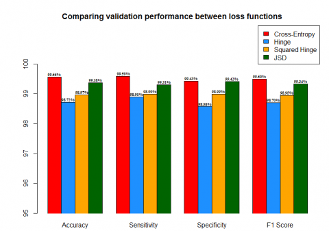
According to Table 1 and Figure 5, cross entropy produces the best validation performance in all four classification measures. Cross entropy’s accuracy surpasses hinge’s accuracy by 0.84%, squared hinge’s by 0.59% and JSD’s by only 0.18%. Similar results are produced for the other three measures, while cross-entropy displays the best performance against the other examined functions. Although, its difference in validation accuracy from JSD function remains small.
Figure 5. Bar plot displaying the validation performance of the examined loss functions, constructed according to the presented results of Table 1
Moreover, we compare the performance of the selected loss functions according to the 813 images that the test set contains. The CNN structure utilizing cross-entropy reached nearly perfect testing capacity in all utilized measures (Figure 6). Moreover, remarkable performance is accomplished from JSD function with 99.33% testing accuracy 99.25% sensitivity and 99.24% f1 score.
Figure 6. Bar plot displaying the testing performance of the utilized loss functions, constructed according to the presented results of Table 2
4.4 Comparison of binary brain tumor classification - detection
In this section, we will compare the accuracy of the other binary classification models that use CNN structures as we mentioned above. By observing Table 3, we could conclude that our method proposes a very reliable model for brain tumor diagnoses, surpassing the performance of other proposed methodologies. Simultaneously, we provide a low complexity structure, avoiding appearance of overfitting and a very short training-validation duration, introducing an innovative approach for modern medicine. The combination of our automated process with the knowledge of an experienced doctor will revolutionize the field of preventive medicine by saving more and more human lives and simultaneously downgrading the threat of death.
The main idea behind this approach is the construction of an economic and automatic classification tool that will aid doctors around the world overcoming the difficulties of a brain tumor diagnosis based on MRI images. Our model trained and validated on MRI images, gives 99.62% testing accuracy using cross-entropy loss function. The nature of our problem demands a low complexity CNN structure to overcome the danger of overfitting that accompanies small datasets. Similar methodology should be applied to various problems in the field of medicine because data collection is usually limited. The extremely short training-validation period needed for our analysis is another signature advantage gained from this economic structure, highlighting the usefulness of simpler mathematical models in real life applications.
We examined the diagnostic efficiency of four loss functions; cross-entropy, hinge, square hinge and Jensen-Shannon divergence. Comparing the performance of the loss functions mentioned above, according to four widely used measures, we validate the appropriateness of cross entropy function, while underlining the capability of an alternative loss function as JSD. The low variability of the resulted accuracy produced from various training and validation splits, ensures the trustworthiness of our model.
[1] De Angelis, L.M. (2001). Brain tumors. New England J. Med, 344(2): 114-123. https://doi.org/10.1056/NEJM200101113440207
[2] Stewart, B.W., Wild, C.P. (2014). World Cancer Report 2014. International Agency for Research on Cancer.
[3] Rosai, J., Ackerman, L.V. (1979). The pathology of tumors, part III: Grading, staging & classification. Cancer Journal for Clinicians, 29(2): 66-77. https://doi.org/10.3322/canjclin.29.2.66
[4] Gladson, C.L., Prayson, R.A., Liu, W. (2010). The pathobiology of glioma tumors. Annual Review of Pathology: Mechanisms of Disease, 5: 33-50. https://doi.org/10.1146/annurev-pathol-121808-102109
[5] Manjunath, S., Sanjay Pande, M.B., Raveesh, B.N., Madhusudhan, G.K. (2019). Brain tumor detection and classification using convolution neural network. International Journal of Recent Technology and Engineering, 8: 34-40. https://doi.org/10.2139/ssrn.3507904
[6] Ramdlon, R.H., Kusumaningtyas, E.M., Karlita, T. (2019) Brain tumor classification using MRI images with K-nearest neighbor method. 2019 International Electronics Symposium, pp. 660-667. https://doi.org/10.1109/ELECSYM.2019.8901560
[7] Vani, N., Sowmya, A., Jayamma, N. (2017). Brain tumor classification using support vector machine. International Journal of Research in Arts and Science, 5: 258-270. https://doi.org/10.9756/BP2019.1002/25
[8] Mathew, A.R., Anto, P.B. (2017). Tumor detection and classification of MRI brain image using wavelet transform and SVM. 2017 International Conference on Signal Processing and Communication (ICSPC), pp. 75-78. https://doi.org/10.1109/CSPC.2017.8305810
[9] Babu, K.R., Deepthi, U.S., Madhuri, A.S., Prasad, P.S., Shammem, S. (2019). Comparative analysis of brain tumor detection using deep learning methods. International Journal of Scientific & Technology Research, 8: 250-254.
[10] Seetha, J., Raja, S.S. (2018). Brain tumor classification using convolutional neural networks. Biomedical & Pharmacology Journal, 11(3): 1457-1461. http://biomedpharmajournal.org/?p=22844.
[11] Kulkarni, S.M., Sundari, G. (2020). Brain MRI classification using deep learning algorithm. International Journal of Engineering and Advanced Technology, 9: 1226-1231.
[12] Pathak, K., Pavthawala, M., Patel, N., Malek, D., Shah, V., Vaidya, B. (2019). Classification of brain tumor using convolutional neural network. Proceedings of the Third International Conference on Electronics Communication and Aerospace Technology, pp. 128-132. https://doi.org/10.1109/ICECA.2019.8821931
[13] Lang, R., Jia, K., Feng, J. (2018). Brain tumor identification based on CNN-SVM model. Proceedings of the 2nd International Conference on Biomedical Engineering and Bioinformatics, pp. 31-35. https://doi.org/10.1145/3278198.3278209
[14] Sert, E., Ӧzyurt, F., Doğanteklin, A. (2019). A new approach for brain tumor diagnosis system: Single image super resolution based maximum fuzzy entropy segmentation and convolutional neural network. Medical Hypotheses, 133: 109413. https://doi.org/10.1016/j.mehy.2019.109413
[15] Ӧzyurt, F., Sert, E., Avci, E., Doğanteklin, E. (2019). Brain tumor detection on Convolutional Neural Networks with neutrosophic expert maximum fuzzy sure entropy. Measurement, 147: 106830. https://doi.org/10.1016/j.measurement.2019.07.058
[16] Ari, A., Hanbay, D. (2018). Deep learning based brain tumor classification and detection system. Turkish Journal of Electrical Engineering & Computer Science, 26: 2275-2286. https://doi.org/10.3906/elk-1801-8
[17] Hossain, T., Shishir, F.S., Ashraf, M., Al Nasim, M.A., Shah, F.M. (2019). Brain tumor detection using convolutional neural network. 1st International Conference on Advances in Science, Engineering and Robotics Technology, pp. 1-6. https://doi.org/10.1109/ICASERT.2019.8934561
[18] Banerjee, S. (2019). Deep radiomics for brain tumor detection and classification from multi-sequence MRI. arXiv preprint 1903.09210v1.
[19] Xu, Y., Jia, Z., Wang, L.B., Ai, Y., Zhang, F., Lai, M., Chang, E.I. (2017). Large scale tissue histopathology image classification, segmentation, and visualization via deep convolutional activation features. BMC Bioinformatics, 18: 281. https://doi.org/10.1186/s12859-017-1685-x
[20] Murali, E., Meena, K. (2019). A novel approach for classification of brain tumor using R-CNN. International Journal of Engineering Applied Sciences and Technology, 4(4): 360-364. https://doi.org/10.33564/IJEAST.2019.v04i04.058
[21] Xu, Y., Jia, Z., Ai, Y., Zhang, F., Chang, E. (2015). Deep convolutional activation features for large scale brain tumor histopathology image classification and segmentation. 2015 IEEE International Conference on Acoustics, Speech and Signal Processing, pp. 947-951. https://doi.org/10.1109/ICASSP.2015.7178109
[22] Mohammed, M., Nalluru, S.S., Tadi, S., Samineni, R. (2020). Brain tumor image classification using convolutional neural networks. International Journal of Advanced Science and Technology, 29: 928-934.
[23] Saxena, P., Maheshwari, A., Maheshwari, S. (2020). Predictive modeling of brain tumor: A deep learning approach. International Conference on Innovations in Computational Intelligence and Computer Vision. https://doi.org/10.13140/RG.2.2.22911.76963
[24] Sajja, V.R., Kalluri, H.K. (2020). Classification of brain tumors using convolutional neural networks over various SVM methods. Ingénierie des Systèmes d’Information, 25(4): 489-495. https://doi.org/10.18280/isi.250412
[25] Das, S., Aranya O.F.M.R.R, Labiba, N.N. (2019). Brain tumor classification using convolutional neural network. 2019 1st International Conference on Advances in Science, Engineering and Robotics Technology (ICASERT), pp. 1-5. https://doi.org/10.1109/ICASERT.2019.8934603
[26] Afshar, P., Plataniotis, K.N., Mohammadi, A. (2019). Capsule networks for brain tumor classification based on MRI images and coarse tumor boundaries. 2019 IEEE International Conferenceon Acoustics, Speech and Signal Processing, pp. 1368-1372. https://doi.org/ICASSP.2019.8683759
[27] Alqudah, A.M., Alquraan, H., Qasmieh, I.A., Alqudah, A., Al-Sharu, W. (2019). Brain tumor classification using deep learning technique - a comparison between cropped, uncropped, and segmented lesion images with different sizes. International Journal of Advanced Trends in Computer Science and Engineering, 8(6): 3684-3691. http://doi.org/10.30534/ijatcse/2019/155862019
[28] Mittal, A., Kumar, D. (2019). AiCNNs (artificially-integrated convolutional neural networks) for brain tumor prediction. EAI Endorse Transactions on Pervasive Health and Technology, 5: 1-18. http://doi.org/10.4108/eai.12-2-2019.161976
[29] Mohsen, H., El-Dahshan, E.A., El-Horbaty, E.M., Salem, A.M. (2017). Classification using deep learning neural networks for brain tumors. Future Computing and Informatics Journal, 3(1): 68-71. https://doi.org/10.1016/j.fcij.2017.12.001
[30] Sajjad, M., Khan, S., Muhammad, K., Wu, W., Ullah, A., Baik, S.W. (2019). Multi-grade brain tumor classification using deep CNN with extensive data augmentation. Journal of Computational Science, 30: 174-182. https://doi.org/10.1016/j.jocs.2018.12.003
[31] Zhou, Y., Li, Z., Zhu, H., Chen, C., Gao, M., Xu, K., Xu., J. (2019). Holistic brain tumor screening and classification based on DenseNet and recurrent neural network. In: Crimi A., Bakas S., Kuijf H., Keyvan F., Reyes M., van Walsum T. (eds) Brainlesion: Glioma, Multiple Sclerosis, Stroke and Traumatic Brain Injuries. BrainLes 2018. Lecture Notes in Computer Science, vol 11383. Springer, Cham. https://doi.org/10.1007/978-3-030-11723-8_21
[32] Sultan, H.H., Salem, N.M., Al-Atabany, W. (2019) Multi-classification on brain tumor images using deep neural network. IEEE Access, 7: 69215-69225. https://doi.org/10.1109/ACCESS.2019.2919122
[33] Ari, A., Alcin, O.F., Hanbay, D. (2020). Brain MR image classification based on deep features by using extreme learning machines. Biomedical Journal of Scientific and Technical Research, 25: 19137-19144. https://doi.org/10.26717/BJSTR.2020.25.004201
[34] Zhao, L., Jia, K. (2016). Multiscale CNNs for brain tumor segmentation and diagnosis. Computational and Mathematical Methods in Medicine, 2016: 1-17. https://doi.org/10.1155/2016/8356294
[35] Wang, J., Perez, L. (2017). The effectiveness of data augmentation in image classification using deep learning Convolutional Neural Networks. arXiv: 1712.04621.
[36] Le Cun, Y., Bengio, Y., Hinton, G. (2015). Deep Learning. Nature, 521: 436-444. https://doi.org/10.1038/nature14539
[37] Wu, J. (2017). Introduction to Convolutional Neural Networks. https://cs.nju.edu.cn/wujx/paper/CNN.pdf.
[38] Szegedy, C., Liu, W., Jia, Y.Q., Sermanet, P., Reed, S., Anguelov, D., Erhan, D., Vanhoucke, V., Rabinovich, A. (2015). Going deeper with convolutions. 2015 IEEE Conference on Computer Vision and Pattern Recognition (CVPR), IEEE, pp. 1-9. https://doi.org/10.1109/CVPR.2015.7298594
[39] Scherer, D., Müller, A., Behnke, S. (2010). Evaluation of pooling operations in convolutional architectures for object recognition. In: Diamantaras K., Duch W., Iliadis L.S. (eds) Artificial Neural Networks – ICANN 2010. ICANN 2010. Lecture Notes in Computer Science, vol 6354. Springer, Berlin, Heidelberg. https://doi.org/10.1007/978-3-642-15825-4_10
[40] Santurkar, S., Tsipras, D., Ilyas, A., Madry, A. (2018). How does batch normalization help optimization? 32nd Conference on Neural Information Processing Systems.
[41] Srivastava, N., Hinton, G., Krizhevsky, A., Sutskever, I., Salakhutdinov, R. (2014). Dropout: A simple way to prevent neural networks from overfitting. Journal of Machine Learnig Research, 15(56): 1929-1958.