Indrajeet Kumar* | Ritesh Kumar Mishra
© 2021 IIETA. This article is published by IIETA and is licensed under the CC BY 4.0 license (http://creativecommons.org/licenses/by/4.0/).
OPEN ACCESS
In this paper, the performance of two linear detectors in multi-user (MU) multiple-input multiple-output (MIMO) systems is investigated. The uplink sum rate and lower bound of channel capacity is derived for both maximum-ratio combination (MRC) and minimum mean square error (MMSE) schemes considering imperfect and perfect channel state information (CSI) conditions. Results show that linear detector performance improves dramatically when the number of base station (BS) users is smaller than that of BS antennas. It is being demonstrated that in the case of imperfect CSI and the number of BS antennas in the conditions of perfect CSI the transmitting power of users can be decreased by the square root of the number of BS antennas. Simulation results show that the MMSE detector outperforms the MRC detector. The results indicated that the system's uplink sum rate is increased by using significantly larger antenna arrays as opposed to just one antenna system. The findings of the Monte-Carlo simulation are very close to the analytical results.
channel capacity, maximum-ratio combining, minimum mean square error, MU multiple input multiple output, spectral efficiency, massive multiple input multiple output
MU MIMO Systems has gained considerably more attention in recent times [1, 2]. In MU MIMO network, a BS equipped with several antennas usually serves the number of user. In general, the BS interacts with each user by orthogonalizing the broadcast channel in a distinct time/ frequency means [3]. Later on MU MIMO having multiple antenna arrays, containing more than hundreds of antennas at the BS, simultaneously joining to several of users, has fascinated more attention in works [4, 5]. Considering large number of users, these systems are mentioned to as massive MIMO or large MU MIMO systems. Design and analysis of massive MIMO system are new interesting topics [6, 7].
In massive MIMO system random variation of the signal can be considered as deterministic, so we can have averaged out the small-scale fading effect. To improve the effectiveness of the massive MIMO system, regular detectors/precoders such as maximum ratio transmission (MRT), MRC and MMSE [8-10] have been considered. Du et al. [11] developed a special technique using full-duplex BS, sequential beamforming through closed or open-loop training for data communication. A new beamforming technique using the MMSE technique called joint spatial division multiplexing is proposed where a MU precoder and a pre-beam former [12-14] are developed consecutively to maximize the sum rate. In MU-MIMO, many users are provided by several antennas. The channel is generally orthogonal for transmission between users and BSs in the various frequency-time environment. The selective decode forward (SD-F) cooperative system analysis is studied in works [15, 16] over time by the selective Nakagami-m fading channel.
At BS Massive MIMO supports a significantly large number of antennas. This improves the reliability and data rate and also one primary technology that enables ultra-high spectral efficiency in 5G wireless networks for multiple users [17-19]. Numerous techniques to minimize the impact of pilot contamination in the massive MIMO system of TDD were explored [20]. The spectral efficiency of network improves as the number of BS antennas increases. The system performance depends upon the number of BS antennas [21]. Ideally, an orthogonal pilot series is allocated among each user. The length of the coherence block, however, limits the system's maximum number of orthogonal pilot sequences. In a multi-cell system that results in the issue of pilot contamination, these small orthogonal pilot sequences have to be re-used [22, 23]. The significant impact of pilot degradation is that the channel estimates generated at the BS are skewed during the uplink training process, leading to increased network interference.
In this work, derivation of uplink capacity bounds for multiple BS antennas is investigated. The simulation result show that for perfect CSI, the transmitted power of each users can be decreased by a factor of 1/NBS as the number of BS antennas NBS increases. Also, for imperfect CSI, each user transmitted power could be decreased by a factor of due to increase in the number of BS antennas NBS. The closed form expression of achievable rates is derived for limited number of BS antennas, considering perfect and imperfect CSI, respectively.
The rest of the paper is organized as follows: The system model for of MU MIMO is discussed in Section 2. In Section 3, the linear detector under examination is systematically derived. Lower capacity bounds in MU MIMO having perfect CSI and imperfect CSI are examined in Section 4. In section 5 energy efficiency and spectral efficiency analysis is being presented. Simulation results are demonstrated in section 6. Section 7 concludes the paper.
MU MIMO system having NBS antennas at BS, and L single-antenna active users is being considered in this work. In analysis it is assumed that between the users and the BS, CSI is perfect. Let us suppose that the channel matrix between the NBS antennas at the BS and the L users be $H \in \mathbb{C}^{N_{B S} \times L}$, where hldenotes the $N_{B S} \times 1$ channel vector between the lth user and the BS, lth represents the column of H Commonly, propagation channels are demonstrated via small scale fading and large-scale fading. Though, in this work, we have considered small scale fading only. The components of H are supposed to be independent and distributed identically Gaussian distributed with $h_{n_{B S}\quad l} \sim \mathbb{C N}(0,1)$, here $n_{B S}=1,2, \ldots, N_{B S}, l=1,2, \ldots, L$. In uplink transmission L users communicate data to the BS (Figure 1).
Figure 1. The BS having antennas supporting twenty of users in a particular cell
Let us assume $y_{l}$ be the data communicated from the lth user having $E\left\{\left|y_{l}\right|^{2}\right\}=1$, here expected value is represented as $E\{.\}$. Meanwhile the identical time/frequency means is being used by the L users, the detected data at the BS is an NBS´1 vector and is the amalgamation of communicated data from all L users, represented as,
$s=\sqrt{\beta} \sum_{l}^{L} h_{l} y_{l}+\eta=\sqrt{\beta} \mathrm{H} y+\eta$ (1)
where, $\eta \in \mathbb{C}^{N_{B S} \times 1}$ represents the additive white noise vector, β represents communicated SNR per user and $y \triangleq\left[y_{1}, y_{2}, \ldots y_{l}, \ldots y_{L}\right]^{T}$. The components of η are supposed to be i.i.d. Gaussian distributed, not depending on H, with $h_{n_{B S}\quad l} \sim \mathbb{C N}(0,1)$ here $n_{B S}=1,2, \ldots, N_{B S}$. The BS can logically identify the communicated data from the L users utilizing information about the channel state information and s the expression given in (1), which represents the multiple access channel, delivers the sum-capacity, expressed as [10],
$C_{s u m}=\log _{2}\left(\operatorname{det}\left(I_{L}+\beta \mathrm{H}^{\mathrm{H}} \mathrm{H}\right)\right)$ (2)
where, the Hermitian operator is represented as $(.)^{H}$. In favourable transmission environments [12], The channel vectors among the users and the BS are pair wisely orthogonal, and from (2), the optimum sum capacity of the uplink transmission is upper constrained by, $C_{s u m, U B} \leq L \log _{2}\left(1+\beta N_{B S}\right)$. Using complex signal processing techniques in the uplink the optimal performance can be obtained, such as MLD. The BS has to check all possible amalgamations of communicated data vectors y with the help of MU MLD, and choices one of them that minimizes the subsequent conditions
$\hat{y}=\arg \min _{y \in Y^{L}}\|s-\sqrt{\beta} \mathrm{H} y\|^{2}$ (3)
where, Y is the limited alphabet of yl, $l \in\{1,2, \ldots, L\}$. The BS has to execute a examine over |Y|L vectors, where |Y| represents the cardinality of set Y. Thus, the complication related with MLD is exponential in relation to L.
To decrease the difficulty of signal processing an alternate linear processing technique is introduced, which is the main objective of this work. Utilizing linear detectors at the BS, s could be fragmented into L streams of data. By multiplying s with W this can be done.
$\tilde{s}=W^{H} s=\sqrt{\beta} W^{H} \mathrm{H} y+W^{H} \eta$ (4)
where, $N_{B S} \times L$ linear detection matrix is represented by W. Subsequently, each one of these data streams is individually decrypted. In this particular situation, L|Y| is the order of detection system complexity. Using (4), the lth stream /component of $\tilde{s}$, which is being utilized in decrypting yl, is given by:
$\tilde{s}_{l}=\sqrt{\beta} w_{l}^{H} h_{l} y_{l}+\sqrt{\beta} \sum_{l^{\prime} \neq l}^{L} w_{l}^{H} h_{l^{\prime}} y_{l^{\prime}}+w_{l}^{H} \eta$ (5)
where, lthcolumn of W is represented as wl. The wanted signal for detection, the inter-user interference and the noise components is represented by first term, second term, final term respectively in (5). The effective noise is the sum of interference plus noise, which is a Random Variable (RV) having variance $\beta \sum_{l^{\prime} \neq l}^{L_{l}}\left|w_{l}^{H} y_{l^{\prime}}\right|^{2}+\left\|w_{l}\right\|^{2}$ and zero mean. Therefore, the detected lthcomponent Signal to Interference-plus-Noise Ratio (SINR) is being given by:
$S I N R_{l}=\frac{\beta\left|w_{l}^{H} h_{l}\right|^{2}}{\beta \sum_{l^{\prime} \neq l}^{L}\left|w_{l}^{H} h_{l^{\prime}}\right|^{2}+\left\|w_{l}\right\|^{2}}$ (6)
First, we concisely present the two orthodox linear MU detectors under examination, MRC and MMSE [9]. The main objective of MRC detector is to maximize the detected SNR of each and every component, while it overlooks the influence of MU interference. The MRC detector that fulfils this situation, Wmrc=H, outcomes in the succeeding detected SINR for the lthstream of data
$S I N R_{m r c, l}=\frac{\beta\left|h_{l}\right|^{4}}{\beta \sum_{l^{\prime} \neq l}^{L}\left|h_{l}^{H} h_{l^{\prime}}\right|^{2}+\left\|h_{l}\right\|^{4}}$ (7)
MMSE detector wishes at minimalizing the Mean Square Error (MSE) between the approximation $W^{H} s$ and the communicated signal y, as follows:
$w_{m m s e}=\arg \min _{w \in \mathbb{C}^{N_ {B S} \times L}} E\left\{\left\|W^{H} s-y\right\|^{2}\right\}$ (8)
Therefore, the detected SINR for the lth stream of data for the MMSE detector, $w_{m m s e}=H\left(H^{H} H+\frac{1}{\beta} I_{L}\right)$ which fulfils such situation, is:
$S I N R_{\text {mmse }, l}=\beta h_{l}^{H}\left(\beta \sum_{i \neq l}^{L} h_{i} h_{i}^{H}+I_{N_{B S}}\right)^{-1} h_{l}$ (9)
We can begin first by amending the explanation of the channel to replicate geometric attenuation and shadow fading as given below:
$g_{n_{B S} l}=h_{n_{B S} l} \sqrt{\xi_{l}}, \quad G=\mathrm{H} D^{1 / 2}$ (10)
where, l=1,2,...,L, nBS=1,2,...,NBS, $[H]_{n_{B S} l}=h_{n_{B S} l}$, L´L diagonal matrix is represented as D, where [D]ll=ξl, and ξk is modelled as the geometric attenuation and shadow fading, which is supposed to be identified a priori, constant over countless periods of coherence time, and not depending on any value of nBS.This supposition is considered acceptable as the distances are considerably higher between the BS and the users than the distance between any two antenna and ξk changes it value very slowly with respect to time.
First of all, we have considered the case when CSI is perfect at the BS. Let channel $N_{B S} \times L$ linear receiver matrix is represented as W. Replacing the new characterization of the channel into (5).
$\tilde{s}_{l}=\sqrt{\beta} w_{l}^{H} g_{l} x_{l}+\sqrt{\beta} \sum_{l^{\prime} \neq l}^{L} w_{l}^{H} g_{l^{\prime}} x_{l^{\prime}}+w_{l}^{H} \eta$ (11)
where, lthcolumn of G is represented as gl. Also, we assumed here the channel to be ergodic in order for each and every symbol to span over numerous realizations of the fast-fading component of G. Hence, the lthuser achievable uplink rate is given as:
$C_{P, l}=E\left\{\log _{2}\left(1+\frac{\beta\left|w^{H} g_{l}\right|^{2}}{\beta \sum_{l^{\prime} \neq l}^{L}\left|w_{l}^{H} g_{l^{\prime}}\right|^{2}+\left\|w_{l}\right\|^{2}}\right)\right\}$ (12)
whenever the BS is having perfect CSI [9], each and every user broadcast power is to be scaled by number of antennas NBS at BS according to $\beta=\frac{E}{N_{B S}}$. Total transmission power for all workstations is supposed to be constant and it is represented as E. Therefore
$\lim _{N_{B S} \rightarrow \text { Infinity }} C_{P, l}=\log _{2}\left(1+\xi_{l} E\right)$ (13)
In MRC detector, W=G, and so, wl=gl. By using (12), we can easily compute the achievable rate for the lthuser as:
$C_{P, l}^{m r c}=E\left\{\log _{2}\left(1+\frac{\beta\left|g_{l}\right|^{4}}{\beta \sum_{l^{\prime} \neq l}^{L}\left|g_{l}^{H} g_{l^{\prime}}\right|^{2}+\left\|g_{l}\right\|^{2}}\right)\right\}$ (14)
After putting $\beta=\frac{E}{N_{B S}}$ into (14), using Jensen’s inequality and by the degree of the curve of $\log _{2}\left(1+\frac{1}{r}\right)$, the achievable rate lower bound would be:
$\tilde{C}_{P, l}^{m r c}=\log _{2}\left(1+\frac{\frac{E}{N_{B S}}\left(N_{B S}-1\right) \xi_{l}}{\frac{E}{N_{B S}} \sum_{l^{\prime} \neq l}^{L} \xi_{l^{\prime}}+1}\right)$ (15)
where, $C_{P, l}^{m r c} \geq \tilde{C}_{P, l}^{m r c}$ and,
$\tilde{C}_{P, l}^{m r c} \triangleq \log _{2}\left(1+\left(E\left\{\frac{\beta \sum_{l^{\prime} \neq l}^{L}\left|g_{l}^{H} g_{l^{\prime}}\right|^{2}+\left\|g_{l}\right\|^{2}}{\beta\left\|g_{l}\right\|^{4}}\right\}\right)^{-1}\right)$ (16)
The lower bound achieved in (15) come together to the similar outcome as in (13) as NBSincreases without limit. Additionally, using the law of large numbers [10] the similar outcome for MMSE detectors can be realized. Note that $\frac{1}{N_{B S}} G^{H} G$ approaches D, as NBSincreases larger. Thus, the performance of MMSE receiver is approaching towards the MRC performance. This indication that for the situation of very large antennas NBSat a BS having perfect CSI, a MU Massive MIMO system with an E/NBS transmission power for every user has an identical efficiency to that of a SISO system with E transmission power, deprived of any kind of intracell interference and fast fading, while decreasing users power by 1/NBS and improving the uplink sum rate by L times.
Now, considering the second situation of BS having imperfect CSI, where the BS wants to approximate the channel matrix, G. This can be performed by utilizing UL pilots in an OFDM systems. Here Tc represents the coherence interval length of symbols, and μ represents the number of pilot codes. The mutually orthogonal pilot series of length μ, which can simultaneously communicate for the period of the coherence interval training duration by the L users. It could be stated by a $\mu \times L$ matrix, $\sqrt{\beta_{p}} \varphi(\mu \geq L)$ that fulfils $\varphi^{H} \varphi=I_{L}$b, where $\beta_{p} \triangleq \mu \beta$. Thus, at the BS, the NBS´μ detected pilot matrix is,
$R_{P}=\sqrt{\beta} G \psi^{T}+\Gamma$ (17)
where, $N_{B S} \times \mu$ noise matrix is represented as Γ, with components that are i.i.d. $\mathbb{C N}$(0, 1). Using R, the MMSE approximation of G is,
$\hat{G}=\frac{1}{\sqrt{\beta_{P}}} R_{P} \psi^{*} \tilde{D}=\left(G+\frac{1}{\sqrt{\beta_{P}}} \Delta\right) \tilde{D}$ (18)
where, the complex conjugate denoted as $(.)^{*}$, $\Delta \triangleq \Gamma \psi^{*}$, and $\widetilde{D} \triangleq\left(\frac{1}{\sqrt{\beta_{P}}} D^{-1}+I_{L}\right)^{-1}$. D has i.i.d. $\mathbb{C N}$(0, 1) components because $\varphi^{H} \varphi=I_{L}$. In the meantime, the method of appraising the channel must be executed on a per-detector antennas basis, the pilot signals independent of large antennas NBS. This information is revealed in all the above results that are obtained and is indicated by $Q \triangleq \hat{G}-G$. From (18), the components of the ithcolumn of Q are random variable with zero means and $\frac{\xi_{i}}{\beta_{P} \xi_{i}+1}$ variances. Also, Q is not depending on $\hat{G}$ due to the attribute of MMSE calculation. The detected BS vector could be stated as:
$\widehat{s}=\hat{w}\left(\sqrt{\beta_{P}} \hat{G} y-\sqrt{\beta_{P}} Q y+\eta\right)$ (19)
Therefore the $l^{t h}$ user detected signal as:
$\widehat{s}_{k}=\sqrt{\beta_{P}} \hat{w}_{l}^{H} \hat{g}_{l} y_{l}+\sqrt{\beta_{P}} \sum_{l^{\prime} \neq l}^{L} \hat{w}_{l}^{H} \hat{g}_{l^{\prime}} y_{l^{\prime}}$
$-\sqrt{\beta_{P}} \sum_{l^{\prime} \neq l}^{L} \hat{w}_{l^{\prime}}^{H} Q_{l^{\prime}} y_{l^{\prime}}+\hat{w}_{l^{\prime}}^{H} \eta$ (20)
where, lth columns of $\hat{W}, \hat{G}$ and Q are represented as $\widehat{w}_{l}, \widehat{g}_{l}$ and $Q_{l^{\prime}}$, respectively. $\hat{W}$ and Q are not depending by virtue of $\hat{G}$ and Q is also self-governing. The first terms of (20) represents the channel estimates and last three term are represented as noise and interference. It is predictable that if there is a drastic reduction in the communicated power per user, there will be a squaring effect as these signals are multiplied simultaneously at the detector. Therefore, it is not practical to decrease broadcast power inversely proportional to NBS, identical to perfect channel state information case [11] proved and advised that a decrease in power only proportionately to 1/NBS could be possible. Therefore, with $\beta=\frac{E}{\sqrt{N_{B S}}}$, and imperfect channel state information that are achieved by MMSE approximation from uplink pilots, we will get:
$\lim _{N_{B S} \rightarrow \text { Infinity }} C_{I P, l}=\log _{2}\left(1+\mu\left(\xi_{l} E\right)^{2}\right)$ (21)
By carrying out same category of investigation as in the perfect channel state information situation, and putting $\beta=\frac{E}{\sqrt{N_{B S}}}$, the achievable rate lower bound for MRC is obtained as given below:
$\tilde{C}_{I P, l}^{m r c}=\log _{2}\left(1+\frac{\mu \frac{E}{\sqrt{N_{B S}}}\left(N_{B S}-1\right) \xi_{l}}{\left(\mu \frac{E}{\sqrt{N_{B S}}}+\frac{1}{\xi_{l}}\right) \sum_{l^{\prime} \neq l}^{L} \xi_{l^{\prime}}+\mu+\frac{\sqrt{N_{B S}}}{E \xi_{l}}+1}\right)$ (22)
As NBS→Infinity, the asymptotic bound achieved on the achievable rate in (22) is identical to the exact limit achieved in (21). We can obtain similar result for the MMSE detectors by using [9].
The energy efficiency is equivalent to the spectral-efficiency divided by the transmitted power. When spectral efficiency grows energy efficiency is decreased and power also increases. So, there is a basic tradeoff between energy efficiency and spectral efficiency. We analyzed the relationship for the uplink of Large MIMO systems in this portion at BS by applying linear receivers in the case of imperfect and perfect CSI. We describe spectral efficiency as:
$\mathfrak{R}_{P}^{A}=\sum_{l=1}^{L} \tilde{\mathfrak{R}}_{P, l}^{A}$ and $\mathfrak{R}_{I P}^{A}=\frac{T-\tau}{T} \sum_{l=1}^{L} \tilde{\mathfrak{R}}_{I P, l}^{A}$ (23)
where, coherence meantime is T and AÎ{mrc, mmse}relates to MRC and MMSE, in symbols. If we avoided large-scale fading effect i.e., D=IL, only MMSE and MRC is taken into consideration. In the case of perfect CSI, from (23) it can be seen that energy efficiency is inversely proportional to spectral efficiency. On the other hand, this rule is not followed for imperfect channel state information. In the upcoming sections the detailed explanation for imperfect CSI has been discussed.
5.1 Maximum-ratio combining
In (23), for MRC, energy efficiency and spectral efficiency is given by,
$\mathfrak{R}_{I P}^{m r c}=\frac{T-\tau}{T} L \log _{2}\left(1+\frac{\tau p_{t u}^{2}\left(M_{B S}-1\right)}{\tau p_{t u}^{2}(L-1)+(L+1) p_{t u}+1}\right)$ (24)
The monotonically increasing function of ptu is $\frac{\partial \mathfrak{R}_{I P}^{m r c}}{\partial p_{t u}}>0 \quad \forall p_{t u}>0 \Re_{I P}^{m r c}$. Thus, energy efficiency is directly proportional to spectral efficiency for low ptu, and the opposite is true for high ptu. This happens because, spectral efficiency undergoes “square effect” when received pilots and received data signal are multiplied. Therefore, at $p_{t u} \ll 1$, and spectral efficiency is $\sim p_{t u}^{2}$. As a result, energy efficiency (spectral efficiency divided by ptu) grows proportionally with ptu. Using Taylor series, $p_{t u} \ll 1$,
$\left.\mathfrak{R}_{I P}^{m r c} \approx \mathfrak{R}_{I P}^{m r c}\right|_{p_{tu=0}}+\left.\frac{\partial^{2} \mathfrak{R}_{I P}^{m r c}}{\partial p_{t u}^{2}}\right|_{p_{t u}=0} p_{t u}^{2}$
$=\frac{T-\tau}{T} L \log _{2}(e) \tau\left(M_{B S}-1\right) p_{t u}^{2}$ (25)
The relation between the energy efficiency and spectral efficiency is given as,
$\eta_{I P}^{m r c}=\sqrt{\frac{T-\tau}{T} L \log _{2}(e) \tau\left(M_{B S}-L\right) \mathfrak{R}_{I P}^{m r c}}$ (26)
By doubling MBS spectral efficiency doubles at $p_{t u} \ll 1$ Energy efficiency grows by 1.5 dB.
5.2 Minimum Mean Square Error
The energy efficiency and spectral efficiency is written from (23), as:
$\eta_{I P}^{m m s e}=\frac{1}{p_{t u}} \mathfrak{R}_{I P}^{m r c} \&$
$\mathfrak{R}_{I P}^{m m s e}=\frac{T-\tau}{T} L \log _{2}\left(1+\frac{\tau\left(M_{B S}-L\right) p_{t u}^{2}}{(L+\tau) p_{t u}+1}\right)$ (27)
Similar to the investigation of maximal ratio combining (MRC), we can also examine that at the low transmitting power ptu, there is improvement in energy efficiency when their will be increase in spectral efficiency. We achieved below expansion of Taylor series in low-ptu regime.
$\mathfrak{R}_{I P}^{m m s e} \approx \frac{T-\tau}{T} L \log _{2}(e) \tau\left(M_{B S}-L\right) p_{t u}^{2}$ and $p_{t u} \ll 1$ (28)
hence,
$\eta_{I P}^{m m s e}=\sqrt{\frac{T-\tau}{T} L \log _{2}(e) \tau\left(M_{B S}-L\right) \Re_{I P}^{m m s e}}$ (29)
Energy efficiency can grow by 1.5 dB when we doubled $\mathfrak{R}_{I P}^{m m s e}$ or MBS when $p_{t u} \ll 1$.
A hexagonal cell having a radius of 1 kilometer is being considered for simulation. In this cell the users are uniformly positioned at random and all the users are rh=100 meters away from the BS. The large-scale fading is displayed via $\beta_{l}=\mathbb{Z}_{l} /\left(r_{l} / r_{h}\right)^{v}$, where $\mathbb{Z}_{l}$ denotes the log-normal random variable having standard deviation σshadow, rl is the distance between the BS and the lth user, and the path loss component is v. For all cases, σshadow=10dB, and v=4.1 has been taken for simulation. It is being assumed her that the communicated signal is modulated with OFDM. Here, all the parameters which are taken are similar to those of LTE standard: Tsd=71.4μs is the symbol duration of OFDM, and Tsd=66.7μs is the useful symbol duration. Hence, the guard interval $T_{g i}=T_{s d}-T_{u s d}=4.7 \mu \mathrm{s}$. Here channel coherence time to be taken as Tc=1 ms. Then, $T_{C I}=\frac{T_{c}}{T_{s d}} \frac{T_{u s d}}{T_{g i}}=200$, where is the number of OFDM symbols in 1 ms coherence interval, and $\frac{T_{c}}{T_{s d}}=15$ is the “frequency smoothness interval” [8].
6.1 For perfect CSI
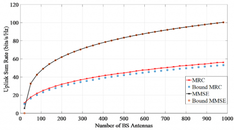
In the case of perfect CSI, simulation is performed to demonstrate the tightness of our planned capacity limits. Figure 2 illustrates the computed uplink sum rate and the suggested analytical bounds for MRC and minimum mean square error (MMSE) detectors with perfect CSI at ptu=11dB. For this case L=20 users is considered. Simulation for L=20 users is done in this case, the coherence interval $T_{C I}=200$, ptu=11dB is the transmitted power by each terminal, and channel propagation variables were σshadow=9dB, and v=4.1. For CSI approximation from uplink pilots pilot sequences of length τ=L is selected. It is being noticed that uplink sum rate for MMSE is much improved than the MRC. From the simulation result it is noticed that when we increase the number BS antennas NBS the difference between uplink sum rate for MRC and MMSE gradually increases. All of the boundaries are very close, particularly at very large NBS. The MMSE receiver is having better performance in comparison to MRC. If the number BS antenna NBS=1000 the uplink sum rate will be 102bits/s/Hz for MMSE.
Figure 2. For perfect CSI, uplink sum rate for distinct number of BS antennas for MMSE and MRC
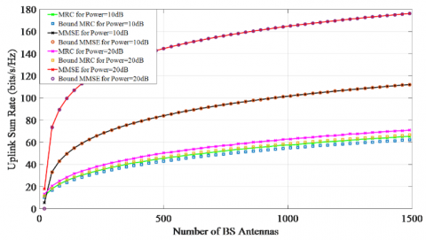
Figure 3. For perfect CSI, uplink sum rate for distinct number of BS antennas for MMSE and MRC at two different power level
In the case of perfect CSI, simulation is performed to demonstrate the tightness of our planned capacity limits. Figure 3 illustrates the computed uplink sum rate and the suggested analytical bounds for MRC and minimum mean square error (MMSE) detectors with perfect CSI at two different power level ptu=10dB and 20dB. Simulation for L=20 users is done in this case, the coherence interval TCI=200, ptu=10dB and 20dB is the transmitted power by each terminal at two different instint of time, and channel propagation variables were σshadow=9dB, and for CSI approximation from uplink pilots pilot sequences of length τ=L is selected. It is being noticed that uplink sum rate for MMSE ptu=20dB is much improved than the uplink sum rate at ptu=10dB. From the simulation result it is noticed that when we increase the number BS antennas NBS the difference between uplink sum rate for MRC and MMSE gradually increases for the same transmitted power. Simulation result also indicates that when we increase the transmitted power for same number of BS antennas NBS the difference between uplink sum rate for MRC or MMSE gradually increases at different power level. All of the boundaries are very close, particularly at very large NBS. The MMSE receiver is having better performance in comparison to MRC at the same transmitted power. If the number BS antenna NBS=1500 the uplink sum rate will be 178bits/s/Hz for MMSE at ptu=20dB.
6.2 For imperfect CSI
In the case of an imperfect CSI, simulation is performed to demonstrate the tightness of our planned capacity limits. Figure 4 illustrates the computed uplink sum rate and the suggested analytical bounds for MRC and minimum mean square error (MMSE) detectors with imperfect CSI at ptu=11dB. Simulation for L=20 users is done in this case, the coherence interval TCI=200, ptu=11dB is the transmitted power by each terminal, and channel propagation variables were σshadow=9dB, and v=4.1. For CSI approximation from uplink pilots pilot sequences of length τ=L is selected. It is being noticed that uplink sum rate for MMSE is much improved than the MRC. From the simulation result it is noticed that when we increase the number BS antennas NBS the difference between uplink sum rate for MRC and MMSE gradually increases. All of the boundaries are very close, particularly at very large NBS. If the number BS antenna NBS=1000 the uplink sum rate will be 71bits/s/Hz for MMSE.
Figure 4. For imperfect CSI, uplink sum rate for distinct number of BS antennas for MMSE and MRC
Figure 5. For imperfect CSI, uplink sum rate for distinct number of BS antennas for MMSE and MRC at two different power level
In the case of perfect CSI, simulation is performed to demonstrate the tightness of our planned capacity limits. Figure 5 illustrates the computed uplink sum rate and the suggested analytical bounds for MRC and minimum mean square error (MMSE) detectors with perfect CSI at two different power level ptu=10dB and 20dB. Simulation for L=20 users is done in this case, the coherence interval TCI=200, ptu=10dB and 20dB is the transmitted power by each terminal at two different instint of time, and channel propagation variables were σshadow=9dB, and v=4.1. For CSI approximation from uplink pilots pilot sequences of length τ=L is selected. It is being noticed that uplink sum rate for MMSE ptu=20dB is much improved than the uplink sum rate at ptu=10dB. From the simulation result it is noticed that when we increase the number BS antennas NBS the difference between uplink sum rate for MRC and MMSE gradually increases for the same transmitted power. Simulation result also indicates that when we increase the transmitted power for same number of BS antennas NBS the difference between uplink sum rate for MRC or MMSE gradually increases at different power level. The MMSE receiver is having better performance in comparison to MRC at the same transmitted power. If the number BS antenna NBS=1500 the uplink sum rate will be 150bits/s/Hz for MMSE at ptu=20dB.
In this work, a detailed investigation of the performance of the linear detectors in very large MU Massive MIMO system is offered. These systems are having improved uplink sum rate, which is expressed in bits/s/Hz uplink sum-rate. This could be of practical use if we are using linear detectors such as MMSE or MRC at the BS having large number of antennas. A MMSE detector outperforms the MRC detector. In general, the performance of MMSE detector is better than the MRC detector. However, MRC could be a practical choice by dropping the power levels, which could finally diminish the cross-talk level. The MRC detectors ignore the influence of cross-talk, and MMSE detector maximizes the detected SINR, therefore, it offers best possible performance. Monte-Carlo simulation results indicates that by using very large antennas, uplink sum rate can be improved in comparison to SISO system.
[1] Gesbert, D., Kountouris, M., Heath, R.W., Chae, C.B., Salzer, T. (2007). Shifting the MIMO paradigm. IEEE Signal Processing Magazine, 24(5): 36-46. https://doi.org/10.1109/MSP.2007.904815
[2] Zhang, Z., Teh, K.C., Li, K.H. (2014). Performance analysis of two‐dimensional massive antenna arrays for future mobile networks. IEEE Transactions on Vehicular Technology, 64(11): 5400-5405. https://doi.org/10.1109/TVT.2014.2384006
[3] Wang, X., Wang, Y., Ma, S. (2015). Upper bound on uplink sum rate for large-scale multiuser MIMO systems with MRC receivers. IEEE Communications Letters, 19(12): 2154-2157. https://doi.org/10.1109/LCOMM.2015.2452909
[4] Marzetta, T.L. (2006). How much training is required for multiuser MIMO. In 2006 Fortieth Asilomar Conference on Signals, Systems and Computers, pp. 359-363. https://doi.org/10.1109/ACSSC.2006.354768
[5] Rusek, F., Persson, D., Lau, B.K., Larsson, E.G., Marzetta, T.L., Edfors, O., Tufvesson, F. (2012). Scaling up MIMO: Opportunities and challenges with very large arrays. IEEE Signal Processing Magazine, 30(1): 40-60. https://doi.org/10.1109/MSP.2011.2178495
[6] Loyka, S., Khojastehnia, M. (2019). Comments on “On favorable propagation in massive MIMO systems and different antenna configurations”. IEEE Access, 7: 185369-185372. https://doi.org/10.1109/ACCESS.2019.2960025
[7] Kumar, I., Sachan, V., Shankar, R., Mishra, R. K. (2020). Performance analysis of multi-user massive MIMO systems with perfect and imperfect CSI. Procedia Computer Science, 167: 1452-1461. https://doi.org/10.1016/j.procs.2020.03.356
[8] Wang, Q., Jing, Y. (2017). Performance analysis and scaling law of MRC/MRT relaying with CSI error in multi-pair massive MIMO systems. IEEE Transactions on Wireless Communications, 16(9): 5882-5896. https://doi.org/10.1109/TWC.2017.2717399
[9] Ngo, H.Q., Larsson, E.G., Marzetta, T.L. (2013). Energy and spectral efficiency of very large multiuser MIMO systems. IEEE Transactions on Communications, 61(4): 1436-1449. https://doi.org/10.1109/TCOMM.2013.020413.110848
[10] Sachan, V., Kumar, I., Bhardwaj, L., Mishra, R.K. (2020). Pairwise error probability analysis of SM-MIMO system employing k–μ fading channel. Procedia Computer Science, 167: 2516-2523. https://doi.org/10.1016/j.procs.2020.03.304
[11] Du, X., Tadrous, J., Sabharwal, A. (2016). Sequential beamforming for multiuser MIMO with full-duplex training. IEEE Transactions on Wireless Communications, 15(12): 8551-8564. https://doi.org/10.1109/TWC.2016.2616338
[12] Huh, H., Caire, G., Papadopoulos, H.C., Ramprashad, S.A. (2012). Achieving" massive MIMO" spectral efficiency with a not-so-large number of antennas. IEEE Transactions on Wireless Communications, 11(9): 3226-3239. https://doi.org/10.1109/TWC.2012.070912.111383
[13] Kumar, I., Sachan, V., Shankar, R., Mishra, R.K. (2018). An investigation of wireless S-DF hybrid satellite terrestrial relaying network over time selective fading channel. Traitement du Signal, 35(2): 103-120. https://doi.org/10.3166/ts.35.103-120
[14] Kumar, S., Singh, A., Mahapatra, R. (2019). Deep learning based massive-MIMO decoder. 2019 IEEE International Conference on Advanced Networks and Telecommunications Systems (ANTS), pp. 1-6. https://doi.org/10.1109/ANTS47819.2019.9118152
[15] Shankar, R., Kumar, I., Kumari, A., Pandey, K.N., Mishra, R.K. (2017). Pairwise error probability analysis and optimal power allocation for selective decode-forward protocol over Nakagami-m fading channels. In 2017 International Conference on Algorithms, Methodology, Models and Applications in Emerging Technologies (ICAMMAET), pp. 1-6. doi:10.1109/ICAMMAET.2017.8186700
[16] Varshney, N., Jagannatham, A.K. (2017). Cognitive decode-and-forward MIMO-RF/FSO cooperative relay networks. IEEE Communications Letters, 21(4): 893-896. https://doi.org/10.1109/LCOMM.2016.2647244
[17] Kumar, I., Mishra, R.K. (2020). An efficient ICI mitigation technique for MIMO-OFDM system in time-varying channels. Mathematical Modelling of Engineering Problems, 7(1): 79-86. https://doi.org/10.18280/mmep.070110
[18] Dai, L., Wang, Z., Wang, J., Yang, Z. (2013). Joint time-frequency channel estimation for time domain synchronous OFDM systems. IEEE Transactions on Broadcasting, 59(1): 168-173. https://doi.org/10.1109/TBC.2012.2219231
[19] Kumar, I., Mishra, R.K. (2020, July). Performance analysis for wireless non-orthogonal multiple access downlink systems. In 2020 International Conference on Emerging Frontiers in Electrical and Electronic Technologies (ICEFEET), pp. 1-6. https://doi.org/10.1109/ICEFEET49149.2020.9186987
[20] Viswanath, P., Tse, D.N.C. (2003). Sum capacity of the vector Gaussian broadcast channel and uplink-downlink duality. IEEE Transactions on Information Theory, 49(8): 1912-1921. https://doi.org/10.1109/TIT.2003.814483
[21] Sachan, V., Shankar, R., Kumar, I., Mishra, R.K. (2019). Performance analysis of SM-MIMO system employing binary PSK and M’ary PSK techniques over different fading channels. Procedia Computer Science, 152: 323-332. https://doi.org/10.1016/j.procs.2019.05.010
[22] Huang, J., Zhou, S., Wang, Z. (2013). Performance results of two iterative receivers for distributed MIMO OFDM with large Doppler deviations. IEEE Journal of Oceanic Engineering, 38(2): 347-357. https://doi.org/10.1109/JOE.2012.2223991
[23] Weingarten, H., Steinberg, Y., Shamai, S. (2006). The capacity region of the Gaussian multiple-input multiple output broadcast channel. IEEE Transactions on Information Theory, 52(9): 3936-3964. https://doi.org/10.1109/TIT.2006.880064