Manthena Narasimha Raju* | Kumaran Natarajan | Chandra Sekhar Vasamsetty
© 2021 IIETA. This article is published by IIETA and is licensed under the CC BY 4.0 license (http://creativecommons.org/licenses/by/4.0/).
OPEN ACCESS
In the area of remote sensing, one of the problems is how high-quality remote sensing images are automatically categorized and classified. There have been many suggestions for alternatives. Amongst these, there are drawbacks of approaches focused on low visual and intermediate visual characteristics. This article, therefore, adopts the deep learning method for classifying high-resolution remote sensing picture scenes to learn semantic knowledge. Most of the existing neural network convolution approaches are focused on the model of transfer training and there are comparatively like hidden Marco models, linear fitting methods, the creation of new neural networks based on the latest high-resolution remote sensing picture data sets. But in this paper, we used a modified backpropagation neural network is proposed to detect the objects in images. To test the performance of the proposed model we use two remote sensing data sets benchmark tests were done. The test-precision, precision, reminder, and F1 scores are all fine with the Assist data collection. The precision, precision, reminder, and F1 score are all enhanced on the SIRI-WHU dataset. The proposed system has better precision and robustness compared to the current approaches including the most conventional methods and certain profound learning methods to scene distinguish high-resolution remote sensing pictures.
remote sensing, object detection, neural network, deep learning, image data
Remote sensing is characterized as the compilation without the physical interaction of information about an item. Knowledge is gained by the identification and evaluation of the surrounding area of modifications that the entity imposes, whether electric, acoustic, or possible. This may involve the emission or variations of an electromagnetic field, acoustic waves that represent or interrupt the object [1], or disruptions to the local gravity or the magnetic potential field because of object presence. Remote sensing is the most general word for electromagnetic data processing techniques. These methods involve the whole electromagnetic range including the microwave's low-frequency radio waves, sub-millimetres, far infrasound, near infrasound, infrared, ultraviolet, x-ray, and gamma-ray zones. The launch of the satellites allows for the collecting of extensive knowledge on planets and their ecosystems, both geographically and synoptically.
Earth-orbiting satellite sensors include knowledge on climate trends and cloud dynamics, the vegetation cover of land areas and its seasonal fluctuations, surface morphology, ocean surface temperature, and near-shore currents. Satellite platforms can track rapidly changing phenomena, particularly in the atmosphere, thanks to their fast-paced coverage ability. The long-lasting and recurrent capacities cause periodic, annual, and long-term changes such as ice cover, desert expansion, and rain forest deforestation to be observed. The extensive synoptic coverage enables geographical and continental characteristics such as flat borders and mountain chains to be examined and analyzed. Planetary probe sensors (orbiters, flybys, surface stations, and rovers) [2, 3] have related knowledge on solar system planets and objects. Until now, one or more spacecraft have explored all planets in the solar system except for Pluto.
The comparative analysis of the planet's properties provides a fresh perspective into the solar system creation and development. By growing the number of satellites initiated and put in space, remote-sensing [4-6] data is one of the powerful data tools used in spatial measurement models. You have simple access to numerous sensors [7-10], spatial resolution [11, 12], radiometric resolution [13], and time resolution [14]. The analysis of their capacities and range, processing, and removing requirements seem necessary. It can also benefit to use photographs captured [15-18] by and digitally transformed satellites [19, 20] with suitable algorithms to mitigate the optical mistake of man as he is unable to interpret and discern the adjustments. Via the implementation of such photos and the grouping of techniques, it emerges that lands that have variations in surfaces and identical reflections may be categorized into one category which paved the way for the first situation which is the grouping of related lands. The high frequency and their coverage capacity are another explanation that has been stressed in the case of satellite images for agricultural studies. Thus, significant occurrences like land-use shifts and plant mantel variations can be identified quickly. This approach plays a crucial role in the research and awareness of natural causes and anomalies. Broad-scale surveys with time-repetition and time-consuming mapping (proper mapping) can lead to ongoing growth and to recognize the climate and its causes.
Therefore, the usage of remote sensing [21, 22] technologies is one of the powerful instruments of environmental and geological research. To recognize the most sustainable resources, including land, water, mines, vegetation’s and destructive phenomena such as flooding, desertification, wind-and-water erosion, sand drift, water, soil salinity, and deforestation, we need constant development. The usage of remote sensing data and satellite data thus leads to lowering prices, saving time, enhancing accuracy and pace. This technology is also progressively required to improve. Data sensing systems for remote sensing is one of the most modern systems for the exploration and extraction of data for earth resource management.
In third and developing world countries, where they have small research budgets and do not have access to data on vegetation mantels, especially mountainous and remote areas, where it is difficult and impossible to access data through satellite sensory services, and in all areas for the observation of the intended features.
The actual maps may be comparable with those produced through the analysis of data obtained from satellites to show the precision and integrity of the data obtained in some regions where reliable and widely agreed data are accessible from farms and fields. The majority of the applications of remote sensing data technologies are based on the measurement and determination of soil surface properties, such as plants, precipitation, minerals, particle, and salinity distribution on the surface and salt layers of soil. In general, the reflecting characteristics of soil vary without foliage, soil color, soil humidity, soil nutrients, and distribution of particles, soil density, and defects in soil surfaces, drainage conditions, various chemical compounds, and soil residential sedimentation. Therefore, remote sensing technologies will play a major part in community growth and planning by rapidly producing land usage data and natural events and temporal adjustments. This Chapter explains the image processing techniques and methods of this report, including the correction and documenting of image data, integration of satellite images, image philters, and image classification.
The identification algorithm based on broad data therefore requires to be investigated urgently. The main technology is to derive the legitimate features of the goal from a great volume of high-score results. It is challenging to apply conventional target detection methods to vast volumes of data. It has an unnatural nature with its reliance. It takes time and depends heavily on the know-how and the properties of the records. The interaction between data can hardly be entirely exploited by the creation of an efficient classifier from a vast number of data. We must then find a way to automatically understand the functions. The most powerful function description is achieved by analyzing a huge volume of data itself. The similarity between the data is exploited to completely create a powerful function extraction and classifier by creating a comparatively complex network framework. More aggressive depth learning has presented a successful ability to automatically derive goal characteristics in recent years. In remote processing of the picture, it can also yield better performance. Machine learning is a broad sector that requires multiple techniques. All these strategies are for particular tasks [11] planned and relevant. What machine learning methodology is most suitable for satellite images to classify artifacts is yet to be established. Two types of guided instruction and unattended training [11] may be categorized in the area of master learning strategies. Under any of these, there are many implementations. Objects for which a satellite image can be derived are defined as perceptible. In this paper, we use a modified backpropagation neural network structure which is to improve the detection of objects from the high-resolution images. The rest of the paper is organized as follows section-2 describes the literature work, section-3 explains the proposed model, section-4 gives details of experiments and section-5 concludes the paper.
Many previous attempts were made to extract entity knowledge automatically from remotely sensed satellite imaging. These attempts have been very complicated, some with relatively straightforward manual interventions and some with complicated methods of analyzing data to try to classify natural and fabricated products. In comparison to true color pictures, the vast majority of the preceding ventures used the peculiar characteristics of multi-spectra and ultra- spectral imagery in their studies. Various researchers tend to use multi-spectral and hyperspectral pictures since several forms of cover and artifacts vary significantly in wavelength. These variations are used to lead to their grouping [1].
This strategy has been used by Jiang et al. [2] to build an "automatic way to delete the river and lake from Landsat's multi-spectral imagery. In several spectral bands, the authors developed many permutations of a 'climate index' for climate characteristics. In the same manner, Lu et al. [3] used NDVI 's study to describe the change to agricultural and pastoral use of the cerrado of Brazil (landscape close to savanna). Some researchers have brought this approach a step further, incorporating multi-spectral photos to detect objects with other observable characteristics. Emerson et al. [1] have been used to generate indices of pixel color variation, topographic entity complexity, and space autocorrelation using the Image Characterizations and Modeling Method (ICAMS) software kit. Those indices were then used to characterize the suburban environment under complex algorithms.
However, Geospatial entity tracking algorithms, as some researchers have shown, are not exclusively confined to aerial imagery. Chiang and Knoblock used target identification and extraction algorithms in their paper "A general approach to the extraction of road-vector data from rast maps". The authors first binned identical colors contained in the map into a substantially restricted color setting due to the high color truth and the distribution of many raster charts, in particular those extracted from physical maps. Following this, a person was requested to pick recognized road characteristics from the chart to classify numerous colors correlated with road characteristics. The authors could extract all the characteristics in a raster, which fit the user-defined road color scheme with this knowledge. Additional automatic post-processing was carried out to delete elements that were morphologically distinct from roads but which had identical colors in the raster. The authors then generated centerlines from the layer of cleaned highways and subsequently processed to correct intersections, which have been skewed during centerline creation.
In comparison to these findings, the aerial imagery of true color was only included in this application since this model necessarily is more extensible so items with such multi-spectral signatures can be separated and low-cost true color imagery can be rendered more usable to the market. Furthermore, training a model of true-color imagery would involve little modification of the core machine learning algorithm to identify other artifacts – only a supplementary algorithm of representations of other entity types should be trained by the user. In this theory, the Terrapattern project develops an online website and utility to classify hundreds of discreet item groups using the same algorithm [4]. But these past works, in particular those of Emerson et al., offer some comprehension of the reasoning behind a machine-learning algorithm named "black box" [1]. It is extremely probable for the hundreds, tens of thousands of parameters that a qualified model can use to provide features such as color variation, geometry, and spatial linkages to other objects.
Computer vision often reveals a drastic rise in demand and ability, coupled with advancement in a wider area of machine learning. Nowadays, machine vision is used for operating vehicles, power monitoring devices, tumor detection, and mobile phones. A special kind of machine learning software, known as artificial neural networks (ANNs), accelerate these developments in computer vision. Although the ANNs are not covered in detail, they are performed utilizing plenty of artificial neurons (essentially discrete algorithms) trained each in a particular role (e.g. color or form determination). These neurons are an excellent way to identify dynamic interactions inside data [5] while they function together [6].
Lee [7] observed that neural networks outperform classical algorithms for image recognition in robotic vision applications. The author started by creating an algorithm that segmented images based on the perceived structure, coloration, and texture, and similar attributes of artifacts within the scene. This algorithm was then used to find items within a space by an isolated robot. Lee also carried out the same procedure using a coevolutionary neural network (CNN) – an architecture specialized in ANN, which was shown in research that was outstanding for the analysis of pictures. The efficiency of target detection improved by 33-50 percent when the robot conducted the same role with CNN architecture.
Song and Yan [8] have also observed that CNNs have strong advantages over conventional image processing approaches. When used for image segmentation tasks, the authors contrasted conventional algorithms and CNNs; that is, sorting various artifacts into pictures. The authors' conventional strategies in image processing involved segmentation in thresholds and segmentation of edges. Segmental threshold algorithms are by far the least computerized and operates by splitting the image into different groups depending on the color value of each pixel in the image. The author's rim detection algorithms segmented a picture by defining places where color, lightness, cloth, or form attributes suddenly modify the horizon as the edge of an entity. The authors analyzed Google's DeepLab CNN architecture after an appraisal of this and other related algorithms. Lee, Song, and Yan also considered CNN to produce stronger outcomes than conventional approaches to computer vision. Interestingly, the authors obtained the strongest results using DeepLab and the conventional segmentation algorithm after the performance was analyzed.
These researchers could not interact with what while the "here" items were discussed in the picture using machine learning. In other terms, they recognized discreet items in the pictures, but could not define what the objects were. This topic is answered by a section of the image processing area known as semantic segmentation. During the semantic segmentation, picture or video items are identified and a class ID such as 'tumors,' 'nerves,' 'path' and the like is allocated. Data are extracted from photographs or recordings, which make for far more possibilities for more analysis or decision-making [9].
The SegNet scene segmentation library, which also uses a CNN architecture, is one of the most popular sanitization tools. SegNet was originally created for classification items inside 'road' scenes in real-time for auto-driving purposes, into semantic groups (e.g., highways, sidewalks, automobiles, pedestrians). In its code, segmentation tasks were performed using parts of SegNet (Development Seed 2017) by numerous GIS-related entity detection initiatives, including Skynet and DeepOSM [10].
The convergence of machine learning and GIS is becoming more and more relevant, with stakeholders in this area varying from major businesses and leading universities to young open-source hobbyists. For e.g., Facebook uses machine learning for OSM road dataset detection, digitalization, and updates commit [11]. The algorithms used by Facebook are proprietary and several private sector firms such as Descartes Laboratories, Space Know, and Orbital Perspective. Fortunately, many scholars can give their methodology and technology to the public through scholarly and open-source networks. Like previous studies utilizing aerial photography, many researchers have implemented techniques for studying panchromatic, multispectral, hyperspectral (hyperspectral), and other sophisticated imaging formats. "Street in your document".
Segmentation of SAR Satellite Images with Deep Fully Convolutional Neural Networks", Henry et al. [12] have used CNNs to exclude road networks from the SAR info. The authors state that conventional approaches are difficult to differentiate roads from cars, rivers, and other characteristics of identical visual and topographical patterns. The FCN8 CNN architecture, utilizing manually annotated pictures (utilizing Google Maps info) as training data, has been used to segment road features. The authors flattened the SAR data to include two-dimensional representations of the neural network. While this has a reduction in the amount of knowledge accessible to the model, the authors notice that unlike optical illusions which can be shielded by cloud shielding, the principal benefit by utilizing SAR knowledge for entity detection is the capacity by SAR sensors to gather data irrespective of prevailing conditions.
In comparison to these researchers, when designing a ground cover segmentation algorithm [13] decided to include all the possible data for their model. The authors used multi-spectral satellite picture measurements of 57 square kilometers (57 picture tiles spanning 1 square kilometer each), the coastal/aerosol bands, blue, green, purple, near-infrared, and shortwave infrarote bands were rendered accessible inside the dataset. They applied this data by building a signal channel for reflection and a flattened version of the RGB. These details were then sent to a U-Net CNN, updated as the original U-net was configured for grey imagery [14], Fischer, and Brox to benefit from an additional depth of detail. Thanks to the restricted training set of 57 photos, the authors were able to achieve reasonably detailed segmentation findings.
Nevertheless, within the Open Source community, there is a pronounced tendency against real-color photography over panchromatic, multi-spectral, hyperspectral, and other specialized imaging groups. This is presumably because of two key factors: true-color imagery from popular outlets such as Google Maps and Mapbox are more readily accessible and current computer study algorithms may be used for true-colored aerial imagery with no significant adjustment. Mnih's doctoral dissertation, "Machine Learning for Aerial Picture Marking" (2013) [23], was one of the most influential and frequently quoted works on true color aerial imaging segmentation. For several initiatives in the open-source world, this paper has been a lodestar. While Mnih 's code and basic methods have been copyrighted since then, this paper is still an incredibly significant discussion on the general design, pre- and post-processing, and model validation.
Here in the proposed model, we use a modified backpropagation neural network to work with the high-resolution remote sensing images. One of the major problems of image processing is the noise/distortion of digitized images during the feature extraction stage often due to binarization. Even though filtering gets rid of a significant part of this digital noise, some of it remains which will affect the accuracy of the recognition/classification process.
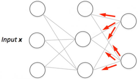
Figure 1. Basic structure of backpropagation neural network
Figure 1 explains the structure of back propagation neural network. One advantage of a backpropagation neural network is that their structure. It is even more effective than CNN because a neuron's output does not necessarily have to be fed back through the entire network, but modified backpropagation neural network rather just through the layer that has unfavorable output. This causes s to converge even faster compared to BP.
3.1 Back propagation learning algorithm
The analogous analogs of an animal's brain axes and their multiple interrelationships by way of synapses are usually conceived as ANNs [21]. The ANN's components are neurons, which are layer-organized (equivalent to biological axons). An ANN has limited input and output layers, each input variable is neuronal and each output class is neuronal. Furthermore, ANNs have secret nodes structured in a supplementary layer or more. The main aspect of an ANN is that all neurons in one layer are bound to another neuron in one layer.
Both layers were adjacent to it and the weights of those links. In conjunction with the normally nonlinear activation function, the weights on ties, which further change values at individual neurons, decide how the input values are mapped to values on the output nodes. Of course, the increase of the number of hidden layers neurons and in particular the inclusion of hidden layers easily improves the possibilities for the description of very complicated judgment limits. Neural networks are normally trained by arbitrarily calculating the weights and then changing the weight and measuring the results on the output nodes. Classification modifications are retained and enhanced; no modifications are scrapped.
ANNs face the difficulty of being late to practice, of delivering not ideal ratings, and being quite overtrained (i.e., delivering over-fit ratings). Besides, a lot of parameters have to be defined by the consumer.
The artificial neurons are then structured in layers, transferring their messages to the outside, and replicating errors. The network receives neurons input in the input layer and the network output is supplied in the output layer by the neurons. One or more unknown intermediate layers can occur. The algorithm for backpropagation uses supervised learning. This implies that the algorithm includes descriptions of the inputs and outputs and then measures the difference between real and predicted results. This error is minimized before the FFNN is conscious of the training data with the backpropagation Algorithm. The preparation starts with random weights, which are modified to reduce the mistake.
In machine learning, a variable y dependent on the vector x of the input variable is always projected. To this end, the input and the output are believed to be essentially usable y= f(x) the predictive model was named. The predictive model is used in supervised learning with training data consisting of instances that are common to both y and x. Examples are accessible pairs (Xi, Yi), where i=1,2,3,.., n, and x vector named element is believed to be composed of. The neural network used for multi-layer feeds is a three-layer network with a secret layer. The input layer is the same as any of the mixed-function vectors corresponds to an irregular or regular output sheet. Each neuron in a specific layer is linked in the next layer to the other neurons. The link of ith to yth neurons is defined by a threshold coefficient of weight and ith neuron. The weight coefficient indicates the extent to which the relation in the neural network is significant. For pattern practicing, the Sigmoid Activation Mechanism is used.
$f(x)=\frac{1}{1+e^{-x}}$ (1)
This is a gradient descent algorithm in which a network is trained before the input vectors and their respective goal vectors can approximate a function. The network uses bias +1 to distinguish input-vectors into irregular and ordinary patients for the concealed layers and a linear feature for the output layers. The cached layers allow the network to generalize. The teaching is carried out with one secret layer and enough neurons to simulate some continuous operation. Layers that are more secret will increase the measurement time contributing to poor rating results. There is no algorithm nor law to select the number of nerve cells in the secret sheet, so the number of neurons concealed is selected manually. The aim is to find the weights between the neurons, which will decide the minimum global feature of the error. The BP network uses an algorithm for descent gradient training that changes the weight for the steepest pitch of the error. Dynamics and arbitrary sets of weights will increase prospects to meet the global minimum.
The training is halted before the error feature is enhanced depending on a fair number of randomly chosen starting weights or after a defined number of iterations. When such inputs are given, the purpose of the training phase is to achieve the desired performance. To reduce the failure, weights must be changed since the error is dependent on the weights. In neural system training, the medium square error function is used and the error function for the performance of each neuron is specified
$E=\frac{1}{n}\sum{\underset{i=1}{\overset{n}{\mathop{\mathop{(y}_{i}-\mathop{t}_{i}}}}\,})^{\wedge}2$ (2)
To correct the original weights, the error function gradient is determined and used to reduce the error functions. The weight is changed by the descending gradient
$\Delta w_{i j}(t+1)=-\eta \frac{\partial E}{\partial W_{i j}}+\alpha \Delta w_{i j}(t)$ (3)
where, E is a warning for malfunction, α is the component of momentum. The α dynamic component makes weight shift momentum. In general, energy enables weight shift over a variety of transition periods to remain. The persistence magnitude is calculated by the component momentum. The enhanced dynamic aspect enhances the persistence of prior changes in the alteration of the new change. The momentum in the back spread algorithm can be useful to speed up the convergence and prevent local minimum amounts. Learning rate μ is a weight-and-bias parameter regulated by practicing a range in an educational method.
3.2 Modified backpropagation algorithm for remote sensing image classification
The learning rate is important to find the real global error gap minimum. The backscatter algorithm pseudo-code is as follows.
For i= 1, 2, 3, ……….n do
Begin
Set the number of neurons in the secret layer
Set Learn rate = 0.01, constant momentum = 0.9, epochmax=1000
Set the weights between [0, +1] and small random values End
Until satisfied do
For each training attribute (xi, yi) train the input & compute the n/w output calculate the MSE
$E=\frac{1}{n}\sum{\underset{i=1}{\overset{n}{\mathop{\mathop{(y}_{i}-\mathop{t}_{i}}}}\,})^{\wedge}2$
If MSE <= acceptable level then stop training
Else, if epoch ≥ epoch max then stop training
Else
Update weights
$E=\frac{1}{n}\sum{\underset{i=1}{\overset{n}{\mathop{\mathop{(y}_{i}-\mathop{t}_{i}}}}\,})^{\wedge}2$
Epoch=epoch+1
End
4.1 Performance metrics
Given any input, a binary classifier predicts either of two outcomes positive, or negative. For the pixel classification problem here, road pixels are considered positive, and background pixels, negative.
The classifier output can be listed as:
▪True Positives (TP): Foreground pixels are classified correctly.
▪True Negatives (TN): Background pixels are classified correctly.
▪False Positives (FP): Background pixels are mistakenly classified as roads.
▪False Negatives (FN): Foreground pixels are mistakenly classified as the background.
These numbers are generally represented in a confusion matrix, as shown below, and the standard metrics used to evaluate a classifier are derived as different ratios from it. The models are then evaluated with these metrics on the initially isolated test data. This gives us a proxy measure of how well the model can generalize.
Two metrics relevant here are Precision and Recall, which are defined as:
Precision $=T P T P+F P$ Recall $=T P T P+F N$
Finally, the best performing models on each dataset are assessed with the F1-score and Intersection Over Union (IOU). These are defined as follows:
$F 1$ Score $=2 * Precision*RecallPrecision + RecallioU =T P TP+F P+F N$
The F1 score is the harmonic mean of Precision and Recall, while IOU is interpreted as the name suggests: the intersection of the actual and predicted values, divided by the union of this set for a specific class.
4.2 Datasets
4.2.1 SIRI-WHU dataset
This Google image dataset covers China's urban areas and is compiled by the RSIDEA (Remote Sensing Intelligent Data Retrieval, Interpretation, and Applications) community.
Figure 2. Example images from SIRI-WHU data set
The dataset for SIRI-WHU consists of 2,400 photographs with 12 scenario groups. There are 200 pictures each of 2 m spatial resolution and 200-pixel scale in each class [24]. The twelve land-use groups involve agricultural, company, port, idle land, manufacturing, meadow, overpass, park, residential wetlands, water [25], and residential wetlands. And though it is shown in Figure 2.
4.2.2 AID dataset
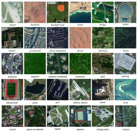
By gathering example photographs from Google Earth photos, Help is a modern, large-scale aerial picture data kit. The latest dataset comprises of 30 separate styles of aerial scenes. The specialists in remote sensing picture analysis mark all pictures. A total of 10000 pictures in Inria 30 groups is accessible in the Help dataset.
Here we are presenting the experimental results of existing and proposed models with respect to accuracy, f-score, precession and recall.
Figure 3. Example images from the AID data set
Figure 4. Accuracy of detecting objects in SIRI-WHU data set
Accuracy is the number of data points of all data points accurately estimated. In more formal words, the number of true positive and genuine negative ones is defined as divided by the number of true positives, true negatives, false positives, and false negatives. More formally, the number of positive and negative truths is described, separated by the number of positive, negative, positive false, and negative truths. Here Figure 3 represents the Accuracy of detecting objects in the SIRI-WHU data set. Besides, the accuracy of detection of objects SIRI-WHU data set is evaluated the proposed and existing Henry, Majid and Merkle have used CNNs to exclude road networks from the SAR info models with different objects. Figure 4 shows how the accuracy of proposed and existing models has performed the detection of objects. The clearly proposed model performs more accurately than existing in the detection of the objects.
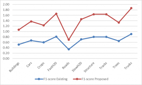
The harmonic mean of precision and reminder is measured as an F-measure, each with the same weighting. The model can be measured using a single ranking, which can be used to define the model’s output and to equate the models both with the consistency and with the reminder. Here Figure 5 represents the F1-score of detecting objects in the SIRI-WHU data set. Besides, the accuracy of the detection of objects SIRI-WHU data set is evaluated by the proposed and existing models with different objects. Figure 5 shows how the F1-score of proposed and existing Henry, Majid, and Merkle have used CNNs to exclude road networks from the SAR info models that are performed detection of objects. The clearly proposed model performs better than existing in the detection of the objects.
Figure 5. F1-score of detecting objects in SIRI-WHU data set
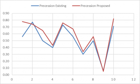
In pattern detection, retrieval, and classification of knowledge (machine learning), correct information (also referred to as positive predictive value) is the fraction of relevant instances among retrieved instances, while retrieval (also called sensitivity) is the fraction of the total number of relevant instances detected. Here Figure 6 represents the precession of detecting objects in the SIRI-WHU data set. Besides, the accuracy of the detection of objects SIRI-WHU data set is evaluated by the proposed and existing models with different objects. Figure 6 shows how the precession of proposed and existing Henry, Majid, and Merkle have used CNNs to exclude road networks from the SAR info models that are performed detection of objects. The clearly proposed model performs better than existing in the detection of the objects.
In pattern detection, retrieval, and classification of knowledge (machine learning), correct information (also referred to as positive predictive value) is the fraction of relevant instances among retrieved instances, while retrieval (also called sensitivity) is the fraction of the total number of relevant instances detected. Here Figure 6 represents the precession of detecting objects in the SIRI-WHU data set. Besides, the accuracy of the detection of objects SIRI-WHU data set is evaluated by the proposed and existing models with different objects. Figure 6 shows how the precession of proposed and existing Henry, Majid, and Merkle have used CNNs to exclude road networks from the SAR info models that are performed detection of objects. The clearly proposed model performs better than existing in the detection of the objects.
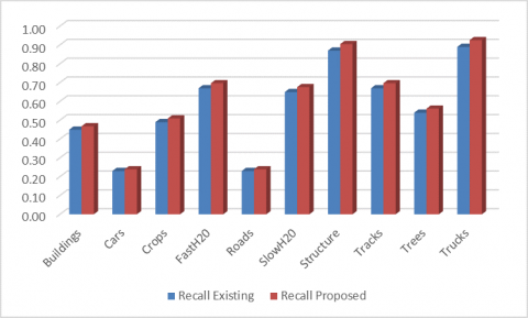
The metric of our intuition is known as a reminder in statistics, or the ability of a model to identify every relevant case in a dataset. The exact concept of recollection is the amount of true positive plus the number of false negatives. Here Figure 7 represents the precession of detecting objects in the SIRI-WHU data set. Besides, the accuracy of the detection of objects SIRI-WHU data set is evaluated by the proposed and existing models with different objects. Figure 7 shows how the recall of proposed and existing Henry, Majid, and Merkle have used CNNs to exclude road networks from the SAR info models are performed detection of objects. The clearly proposed model performs better than existing in the detection of the objects.
Figure 6. Precession of detecting objects in SIRI-WHU data set
Figure 7. Recall of detecting objects in SIRI-WHU data set
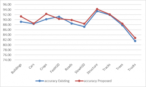
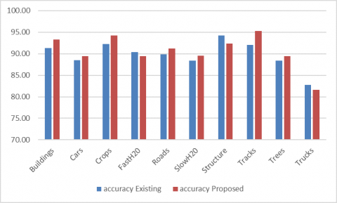
Accuracy is the number of data points of all data points accurately estimated. In more formal words, the number of true positive and genuine negative ones is defined as divided by the number of true positives, true negatives, false positives, and false negatives. More formally, the number of positive and negative truths is described, separated by the number of positive, negative, positive false, and negative truths. Here Figure 8 represents the Accuracy of detecting objects in the AID data set. Also, the accuracy of the detection of objects AID data set is evaluated by the proposed and existing models with different objects. Figure 8 shows how the accuracy of proposed and existing Henry, Majid, and Merkle have used CNNs to exclude road networks from the SAR info models that are performed detection of objects. The clearly proposed model performs more accurately than existing in the detection of the objects.
In pattern detection, retrieval, and classification of knowledge (machine learning), correct information (also referred to as positive predictive value) is the fraction of relevant instances among retrieved instances, while retrieval (also called sensitivity) is the fraction of the total number of relevant instances detected. Here Figure 9 represents the precession of detecting objects in the SIRI-WHU data set. Besides, the accuracy of the detection of objects SIRI-WHU data set is evaluated by the proposed and existing models with different objects. Figure 9 shows how the precession of proposed and existing Henry, Majid, and Merkle have used CNNs to exclude road networks from the SAR info models that are performed detection of objects. The clearly proposed model performs better than existing in the detection of the objects.
Figure 8. Accuracy of detecting objects in the AID data set
Figure 9. Precession of detecting objects in the AID data set
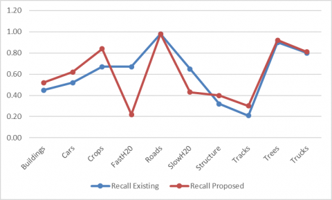
The metric of our intuition is known as a reminder in statistics, or the ability of a model to identify every relevant case in a dataset. The exact concept of recollection is the amount of true positive plus the number of false negatives. Here Figure 10 represents the precession of detecting objects in the AID data set. Also, the accuracy of the detection of objects AID data set is evaluated by the proposed and existing models with different objects. Figure 10 shows how the recall of proposed and existing Henry, Majid, and Merkle have used CNNs to exclude road networks from the SAR info models that are performed detection of objects. The clearly proposed model performs better than existing in the detection of the objects.
Figure 10. Recall of detecting objects in the AID data set
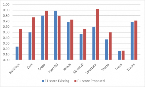
Figure 11. F1-score of detecting objects in the AID data set
The harmonic mean of precision and reminder is measured as an F-measure, each with the same weighting. The model can be measured using a single ranking, which can be used to define the model's output and to equate the models both with the consistency and with the reminder. Here Figure 11 represents the F1-score of detecting objects in the AID data set. Also, the accuracy of the detection of objects AID data set is evaluated by the proposed and existing models with different objects. Figure 11 shows how the F1-score of proposed and existing Henry, Majid, and Merkle have used CNNs to exclude road networks from the SAR info models that are performed detection of objects. The clearly proposed model performs more accurately than existing in the detection of the objects.
This paper presents a method for remote sensing image classification of high-resolution remote sensing images. For the problem of limited data of the existing high-resolution remote sensing datasets, the multi-view scaling strategy is adopted for data amplification, to improve the classification accuracy. In addition to that one of the major problems of image processing is noise/distortion of digitized images during the feature extraction stage often due to binarization. Even though filtering gets rid of a significant part of this digital noise, some of it remains which will affect the accuracy of the recognition/classification process. In this paper, we used the modified backpropagation neural network the major advantage of modified backpropagation neural network is that their structure. It is even more effective than CNN because a neuron's output does not necessarily have to be fed back through the entire network, but modified backpropagation neural network rather just through the layer that has unfavorable output. This causes s to converge even faster compared to BP. To verify the effectiveness of the proposed method, experiments were performed on the SIRI-WHU dataset and the AID dataset. To comprehensively evaluate the proposed method, the evaluation indexes in this paper include accuracy, precision, recall, and F1-score. Compared with the traditional methods and deep learning methods, the proposed method has great advantages.
[1] Emerson, C.W., Lam, N.S.N., Quattrochi, D.A. (2005). A comparison of local variance, fractal dimension, and Moran's I as aids to multispectral image classification. International Journal of Remote Sensing, 26(8): 1575-1588. https://doi.org/10.1080/01431160512331326765
[2] Jiang, H., Feng, M., Zhu, Y., Lu, N., Huang, J., Xiao, T. (2014). An automated method for extracting rivers and lakes from Landsat imagery. Remote Sensing, 6(6): 5067-5089. https://doi.org/10.3390/rs6065067
[3] Lu, D., Hetrick, S., Moran, E., Li, G. (2012). Application of time series Landsat images to examining land-use/land-cover dynamic change. Photogrammetric Engineering and Remote Sensing, 78(7): 747-755. https://doi.org/10.14358/PERS.78.7.747
[4] Levin, G., Newbury, D., McDonald, K., Alvarado, I., Tiwari, A., Zaheer, M. (2016). Terrapattern: Open-ended, visual query-by-example for satellite imagery using deep learning. 2016. Available online: http://terrapattern.com, accessed on 10 March 2020.
[5] Samer, H., Rishi, K., Chris, R. (2015). Using convolutional neural networks for image recognition. Cadence IP.
[6] Schmidhuber, J. (2015). Deep learning in neural networks: An overview. Neural Networks, 61: 85-117. https://doi.org/10.1016/j.neunet.2014.09.003
[7] Lee, A. (2015). Comparing deep neural networks and traditional vision algorithms in mobile robotics. Swarthmore University.
[8] Song, Y.H., Hao, Y. (2017). Image segmentation algorithms overview. 2017 Asia Modelling Symposium (AMS), Kota Kinabalu, Malaysia, pp. 103-107. https://doi.org/10.1109/AMS.2017.24
[9] Shuai, B., Liu, T., Wang, G. (2016). Improving fully convolution network for semantic segmentation. arXiv preprint arXiv:1611.08986. https://arxiv.org/pdf/1611.08986.pdf.
[10] Andrew, L.J. (2017). DeepOSM. https://github.com/trailbehind/DeepOSM, accessed on August 20, 2020.
[11] Patel, D., Gao, M. (2017). OSM @ Facebook. http://2017.stateofthemap.org/2017/ai-assisted-road-tracing-for-openstreetmap/, accessed on August 20, 2020.
[12] Henry, C., Azimi, S.M., Merkle, N. (2018). Road segmentation in SAR satellite images with deep fully convolutional neural networks. IEEE Geoscience and Remote Sensing Letters, 15(12): 1867-1871. https://doi.org/10.1109/LGRS.2018.2864342
[13] Iglovikov, V., Mushinskiy, S., Osin, V. (2017). Satellite imagery feature detection using deep convolutional neural network: A Kaggle competition. arXiv preprint arXiv:1706.06169.
[14] Ronneberger, O., Fischer, P., Brox, T. (2015). U-net: Convolutional networks for biomedical image segmentation. In International Conference on Medical Image Computing and Computer-Assisted Intervention, pp. 234-241. Springer, Cham. https://doi.org/10.1007/978-3-319-24574-4_28
[15] Arizona, U.O. (2005). Growth secrets of Alaska's mysterious field of lakes. https://www.sciencedaily.com/releases/2005/06/050627233623.htm, accessed on August 20, 2020.
[16] Unnikrishnan, R., Pantofaru, C., Hebert, M. (2007). Toward objective evaluation of image segmentation algorithms. IEEE Transactions on Pattern Analysis and Machine Intelligence, 29(6): 929-944. https://doi.org/10.1109/TPAMI.2007.1046
[17] Vance, A. (2017). The Tiny Satellites Ushering in the New Space Revolution. Bloomberg Businessweek, 29.
[18] Walia, A.S. (2017). Types of optimization algorithms used in neural networks and ways to optimize gradient descent. Towards Data Science. https://towardsdatascience.com/types-of-optimization-algorithms-used-in-neural-networks-and-ways-to-optimize-gradient-95ae5d39529f.
[19] Topher, W. (2018). The fight against illegal deforestation with TensorFlow. https://blog.google/topics/machine-learning/fight-against-illegal-deforestation-tensorflow.
[20] Yu, S., Jia, S., Xu, C. (2017). Convolutional neural networks for hyperspectral image classification. Neurocomputing, 219: 88-98. https://doi.org/10.1016/j.neucom.2016.09.010
[21] Zhou, B., Khosla, A., Lapedriza, A., Oliva, A., Torralba, A. (2016). Learning deep features for discriminative localization. 2016 IEEE Conference on Computer Vision and Pattern Recognition (CVPR), Las Vegas, NV, USA, pp. 2921-2929. https://doi.org/10.1109/CVPR.2016.319
[22] Zou, K.H., Warfield, S.K., Bharatha, A., Tempany, C.M., Kaus, M.R., Haker, S.J. (2004). Statistical validation of image segmentation quality based on a spatial overlap index1: Scientific reports. Academic Radiology, 11(2): 178-189. https://doi.org/10.1016/S1076-6332(03)00671-8
[23] Volodymyr, M. (2013). Machine learning for aerial image labeling. PhD Thesis, Graduate Department of Computer Science, University of Toronto.
[24] IBM. (2017). 10 Key Marketing Trends for 2017. IBM. https://www-01.ibm.com/common/ssi/cgi-bin/ssialias? htmlfid=WRL12345USEN, accessed on September 23, 2017.
[25] Jean, N., Burke, M., Xie, M., Davis, W.M., Lobell, D.B., Ermon, S. (2016). Combining satellite imagery and machine learning to predict poverty. Science, 353(6301): 790-794. https://doi.org/10.1126/science.aaf7894