Mohammad Keivani* | Jalil Mazloum | Ezatollah Sedaghatfar | Mohammad Bagher Tavakoli
© 2020 IIETA. This article is published by IIETA and is licensed under the CC BY 4.0 license (http://creativecommons.org/licenses/by/4.0/).
OPEN ACCESS
The main purpose of this research is to apply image processing for plant identification in agriculture. This application field has so far received less attention rather than the other image processing applications domains. This is called the plant identification system. In the plant identification system, the conventional technique is dealt with looking at the leaves and fruits of the plants. However, it does not take into account as a cost effective approach because of its time consumption. The image processing technique can lead to identify the specimens more quickly and classify them through a visual machine method. This paper proposes a methodology for identifying the plant leaf images through several items including GIST and Local Binary Pattern (LBP) features, three kinds of geometric features, as well as color moments, vein features, and texture features based on lacunarity. After completion of the processing phase, the features are normalized, and then Pbest-guide binary particle swarm optimization (PBPSO) is developed as a novel method for reduction of the features. In the next phase, these features are employed for classification of the plant species. Different machine learning classifiers are evaluated including k-nearest neighbor, decision tree, naïve Bayes, and multi-SVM. We tested our proposed technique on Flavia and Folio leaf datasets. The final results demonstrated that the decision tree has the best performance. The results of the experiments reveal that the proposed algorithm shows the accuracy of 98.58% and 90.02% for the "Flavia" and "Folio" datasets, respectively.
plants, GIST, best-guide binary particle swarm optimization, geometrics, machine learning
This research is aimed to apply image processing for plant identification in agriculture. Researchers have paid less attention to this application field rather than the other image processing applications fields. This is called the plant identification system. Many interested researchers have accomplished a lot of researches in various fields comprising meteorology, medicine and especially agriculture [1].
Therefore, there is a considerable demand for development of an automated tool with the capability of identifying species of plants. It helps to expedite their identification. This tool can be very useful for experienced botanists and farmers.
Automatic detection of plants is taken into account as an important research topic for monitoring agricultural crop field. The application of the image processing technique is tremendously expanded for detection of plant species in agriculture. There are various methods for classification purposes such as k-nearest neighbor (KNN) classifier, Probabilistic Neural Network (PNN), Support Vector Machine (SVM).
This paper is developed to propose a novel, comprehensive and hybrid method for classification of plants with respect to leaf images. In this study, our main contribution revolves around feature extraction. The shapes, colors and strong textures features lead to improvement in the accuracy of the proposed method.
We have attempted to capture various items for the leaf including shape, color, vein, and texture. To perform the analysis, we initially used GIST and Local Binary Pattern (LBP) features, three kinds of geometric features, as well as color moments, vein features, and texture features based on lacunarity. The second phase is associated with normalization of the features. In the third phase, Pbest-guide binary particle swarm optimization (PBPSO) is utilized as a new method for reduction of the features. Thereafter, the features are employed to classify the leaf images for different plant species. Various machine learning classifiers are evaluated including decision tree, multi-SVM, naïve Bayes, and k-nearest neighbor. We tested our developed technique on Flavia and Folio leaf datasets. By consideration of the proposed method, the performance is improved based on the accuracy criteria.
An algorithm was developed for detection of plant species in leaf images using vector support [1]. This algorithm is dealt with several steps including preprocessing (it includes boundary enhancement), feature extraction (it includes DMF) and structural features. This method improves the efficiency of the support vector machine for detecting leaf species. This method is tested on both Flavia and local datasets. This classification has the least runtime on the Flavia dataset.
The visual recognition of leaf types may be simple for a botanist, but it is a complex and computationally expensive task for a machine. Wu et al. [2] proposed an efficient algorithm for plant classification. They have considered 32 types of plants. Different shape features have been used encompassing aspect ratio, leaf area, diameter of different vein properties. The accuracy of this method was determined 90.31%. Kadir et al. [3] considered a study to combine the texture, color and texture characteristics using PNN method.
Zheng and Wang [4] introduced a feature extraction method with the capability of identifying several plants, but it was not able to extract the shape features in specific types. Bhardwaj et al. [5] proposed a method with the capability of extracting the shape features. The extracted features are included in features convexity of region, volume fraction and inverse difference moment. Fourier descriptors, morphological characteristics, and mass-shaping characteristics were considered to identify the plants [6]. Geometric morphological characteristics and serrated features were utilized to recognize the plant species with considerable yield. According to Choras [7], texture is taken into account as a powerful regional descriptor that helps to detection process. Various textural features are comprised of Gabor Filter, Local binary pattern (LBP) and Gray-level occurrence matrices (GLCMs). Other methods use the fractals to get texture features. Fractals have been represented for texture classification [8]. A method was proposed to evaluate the number of 32 plant species in leaf images using improved KNN [9].
Singh et al. [10] applied different classifiers for various shape features. In this approach, different geometrical, morphological and vein features were investigated for leaf using PNN classifier. PCA was employed to reduce the extracted features. The accuracy of this method is ascertained 91%.
Gwo and Wei [11] suggested a method by considering several steps. In the first step, leaf contours were calculated, and then key points were selected. In the next step, the fuzzy score algorithm was devoted to manage histogram differences for similar species lengths. The Bayes classifier was used to classify this method.
Islam et al. [12] used the synthetic tissue features for identifying plant species in leaf images. These features were involved in Local Binary Pattern (LBP) and Histogram of Oriented Gradients (HOG). In this case, the extracted features were classified by using the SVM. The accuracy of the features extracted by HOG and SVM classification with respect to cells of 2 x 2, 4 x 4 and 8 x 8 are dealt with 77.5%, 81.25% and 85.31, respectively. By application of LBP and SVM classifier, the accuracy of this method is specified 40.6%. Also, application of the combined HOG and LBP features with the same classification (i.e. SVM) gives the accuracy of 91.25%. Experimental results reveal that HOG + LBP feature extraction through SVM is more accurate than HOG and LBP individually.
A three-step method was proposed for leaf species identification [13]. These steps are comprised of pre-processing, feature extraction and classification. Preprocessing step is the way to enhance the image before processing. In the next step, feature extraction is achieved based on the color and shape of the image. This property is evaluated for ANN and KNN, and then these are compared to each other. Flavia dataset was used for experimental tests. In this regard, the number of 1907 leaf samples were tested. The samples were involved in 33 different plant species. The accuracy of this method by application of ANN is obtained 93.3%.
The proposed method involves in implementing the invariant Fourier Transform (SIFT) algorithm for leaf detection considering the value of key descriptors [14]. The second method deals with identifying and classifying the corner-centered axis. To do this, Mean Projection algorithm was used.
Previous studies on classification of plant species based on leaf images are often problematic. For instance, in some studies, such as PNN-based classification, only some features, including shape and vein, have been extracted, which reduces accuracy. Furthermore, in the Fourier models due to the sinusoidal smooth states for the sharpened leaves, appropriate properties are not extracted. In addition, there are limitations in feature extraction since they do not exhaustively extract all features. For this reason, in order to overcome the above mentioned problems, different features such as shape, color, texture, and veins are considered in the proposed method.
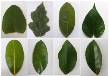
To test the proposed method, Flavia dataset has been utilized, which can be downloaded from the link http://flavia.sourceforge.net [2]. The dataset contains 1600 images of 32 species of plants. Also, Folio Dataset consists of 20 photos of leaves for each of the 32 different species [9]. The leaves were taken from plants in the farm of the University of Mauritius and its nearby locations. To achieve the dataset, it is available at http://archive.ics.uci.edu/ml/datasets/Folio. In this research, the proposed method was tested on 640 leaves belonging to 32 different species of plants. Figure 1 depicts the leaf images for Folio dataset.
Figure 1. Folio dataset leaf images
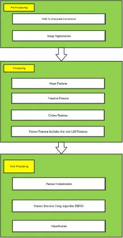
Our proposed algorithm consists of three main phases: (1) preprocessing phase, which deals with converting RGB image into Grayscale and image segmentation) (2) processing phase, which uses the shape features, venation features, color features and texture features including gist and LBP features (3) post processing phase, which develops a new method for feature selection tasks like Pbest-guide binary particle swarm optimization (PBPSO).This method can select the potential features for improvement in the classification accuracy. The proposed framework is shown in Figure 2.
Figure 2. Proposed algorithm for this study
4.1 Leaf image pre-processing and segmentation phase
Pre-processing is considered as an important phase in the image recognition system. The proposed method uses the Flavia dataset containing images with a fixed white background. Therefore, we utilized the pre-processing and segmentation methods, which have been provided by Saleem et al. [15]. In these images, all images dealing with Flavia dataset are converted to 800 x 600 size, whereas the images are halved in the Folio datasets. The segmentation process involves in separating the leaf from its background. Extracting your area of interest (ROI) can be tricky, because the background has indistinct content that is not the case in the proposed method. However, advanced segmentation algorithms can be evolved to exactly extract the ROI for better extraction from desirable features in the Flavia dataset. To make the ROI segmentation, the background of each leaf is white and clear. Color images from the RGB color space are converted to LAB. In this color space, the parameter L represents the brightness intensity, a and b are color-dependent values. In this way, the L layer is initially processed for further processing. The image is then converted to binary using the Otsu threshold method [15].
To extract shape features, we only need the leaf boundary. Figure 3 indicates the binary leaf image with a 3 × 3 Laplace operator. It is processed to smooth the edges of the leaf and adjust the small spots, as well. The preprocessing and segmentation phases are shown in Figure 4. Where, R, G and B denote the red, green and blue channels, respectively. Figure 4(a) shows a sample color image and Figure 4(b) displays Gray image, representing chromatic filter.
Figure 3. Application of Laplacian operator for smoothing leaf edges of the binaries intensity image
Figure 4. Results of pre-processing and segmentation processes for our proposed algorithm
As shown in Figure 4, in the pre-processing stage, the colored input image is converted into a black and white image. Then, the black and white image is converted to binary using the Otsu threshold operation. In the final step, the Laplacian operation is performed on this binary image.
Due to the high quality of the images in the datasets, particularly Flavia, we do not need an algorithm to reduce and enhance the image quality. In addition, the noise level after the application of the Laplacian filter has slightly decreased. Finally, the operations are related to the processing of Flavio’s datasets, and the same operation is done on the Folio images.
4.2 Processing phase
In the research, the features were extracted from shape, color, vein, and texture of the leaf. The following sections describe all of the applied features for identification system.
4.2.1 Shape features
In this section, the geometrical features are used for the identification system. These features are defined as below.
(i): Leaf length: the length of a leaf is concerned with the pixel distance between the ends of the main axis. It is indicated by the abbreviation L.
(ii): Leaf width: the minor-axis length of a leaf is dealt with the pixel distance between the minor-axis endpoints. It is denoted by W.
(iii): Leaf area: the area is characterized as the number of pixels at the leaf surface. It is denoted by A.
(iv): Leaf perimeter: the perimeter of a leaf is associated with the number of pixels counted in the leaf boundary. It is denoted by P.
(v): Rectangularity: it is the measure of the likeness between a rectangle and the leaf shape. It is calculated by $\frac{A}{L \times W}$, where L, W, and A are coincided with the length, width and area of leaf, respectively.
(vi): Diameter: If two points of leaf are considered, they are called the longest distance between them. It is denoted by D.
(vii): Convex hull information: a convex-hull is formed using the boundary points of the leaf. The convex-hull is approximately computed and the number of vertices is extracted.
(viii): Aspect ratio: aspect ratio is introduced as an important criterion, which measures the ratio of leaf length and leaf width A = L/W, where L, W, and A are the length, width and area of leaf, respectively.
(ix): Elongation: elongation can be defined as length in width $\frac{L}{W}$, where L and W are concerned with length and width of leaf, respectively.
(x): Longitudinal spreading: longitudinal spreading can be defined as perimeter to length of the leaf as P/L, where P and L are perimeter and length of leaf, respectively.
(xi): Cross-sectional spreading: it results in division of length and width by the leaf Perimeter of the leaf (i.e. P/(L×W)).
(xii): Solidity: it is considered as the ratio between the area of the leaf A and the area of its convex hull Ac. Solidity of the leaf is calculated as: $\frac{A}{A_{c}}$.
(xiii): Roundness: Roundness is calculated as roundness $=\frac{4 \pi A}{P^{2}}$.
(xiv): Narrow factor: narrow factor of the leaf is formulated as: $\frac{D}{L_{p}}$, where D is diameter of the leaf and Lpis length.
(xv): Eccentricity: eccentricity of the leaf is calculated as: L/(W).
4.2.2 Vein features
Vein features can be extracted by using morphological opening. This operation is performed on the gray scale image with respect to flat, disk-shaped structuring element of radius (e.g. 1, 2 and 3) and subtracted remained image by the margin. Based on that vein, the number of 4 features are calculated by Eq. (1).
$V_{1}=\frac{A_{1}}{A} \quad V_{2}=\frac{A_{2}}{A} V_{3}=\frac{A_{3}}{A}$ (1)
In this case, V1, V2 and V3 represent features of the vein, A1, A2, and A3 express sum of pixels for the vein, and A denotes sum of pixels for the section of the leaf.
4.2.3 Texture features
This section developed to address the available techniques for texture feature extraction. This approach is considered for identification of leaf plant using GIST and LBP texture features. These features are defined through the next sections.
(1) GIST
In recent years, there has been a tendency to use general features for classification of images. General features are taken into consideration as powerful tools, which are used to classify different types of images. The gist feature vector is known as one of the most commonly used features for identifying similar objects in different images.
This paper investigates a novel approach for recognition of plant species using GIST texture. This technique is very suitable for images of the same type features. In this technique, image is divided into several blocks.
The blocks are processed using Gabor filters at different scales and different directions. Then, average of the calculated results is gained for different regions. Thus, the required features information is reached [16]. Perform convolution operation on different portions in order, and then integrate the results to obtain global GIST feature of the image. Suppose that the original image to be processed has the size of M×N.
Firstly, divide it into $n_{b l} \times n_{b l}$ blocks. Each block represents a zone. $n_{s}=n_{b l} \times n_{b l}$ is used to record the total number. The different blocks of the image are labelled and denoted by Bbl , where $\mathbf{i}=1, \ldots, \mathbf{n}_{s}$. Each block is in the same size of $\bar{M} \times \bar{N}$. This is done for ease of calculation and processing.
In the problem of leaf image classification, the proposed method considers the gist feature vector as the basis for classification. To achieve the purpose, a number of Gabor filters are defined in different directions and scales. Convolution is carried out between filters and the original image.
The Gabor filter is a linear and local filter. The convolution core of the Gabor filter is a product of a complex exponential and Gaussian functions. Gabor filters can be very good for detecting texture and edge features if they are properly tuned. Another feature of Gabor filters is related to their high resolution. This means that their response is both local and customizable in both location and frequency domains. The mother wavelet of Gabor filter is defined as follows:
$\mathrm{g} \mathrm{x}, \mathrm{y}=\frac{1}{2 \Pi \sigma_{\mathrm{x}} \sigma_{y}} \exp \left[-\left(\frac{\mathrm{x}_{\theta}^{2}}{\sigma_{\mathrm{x}}}+\frac{\mathrm{y}_{\theta}^{2}}{\sigma_{y}}\right)\right] \times \cos \left(2 \Pi \mathrm{f}_{\mathrm{c}} \mathrm{x}+\varphi\right)$ (2)
where, $\sigma_{x}$ is standard deviation of Gaussian function in $x$ direction along the filter that determines the bandwidth of the filter, $\sigma_{y}$ is standard deviation of Gaussian function across the filter that controls the orientation selectivity of the filter, $f_{c}$ is the central frequency of pass band and $\varphi$ is orientation of the filter. An angle of zero gives the filter response to a vertical feature. Transform the mother wavelet mathematically, and then set of Gabor filter can be obtained in different scales and directions. It is formulated by Eq. (3)
$\left\{\begin{array}{c}\mathrm{g}_{\mathrm{m}, \mathrm{n}}(\mathrm{x}, \mathrm{y})=\mathrm{a}^{-\mathrm{m}}\left(\mathrm{g}\left(x^{\prime}, y^{\prime}\right)\right), \mathrm{a}>1 \\ x^{\prime}=a^{-m}(x \cos \theta+y \sin \theta) \\ y^{\prime}=-x \sin \theta+y \cos \theta \\ \theta=\frac{n \pi}{n+1}\end{array}\right.$ (3)
where, $a^{-m}$ denotes the scale factor, θ describes the rotation angle, m denotes the number of scales, and n denotes the number of directions. There is m×n Gabor filters after the calculation. Firstly, the same processing is performed on the various regions in the original image, and then the cascade operation is adopted. It results in the Gist feature of the image, which formulated as follows:
$\mathrm{G}_{\mathrm{i}}^{\mathrm{bl}}(\mathrm{x}, \mathrm{y})=\operatorname{cat}\left(\mathrm{I}(\mathrm{x}, \mathrm{y})^{*} \mathrm{g}_{\mathrm{mm}}(\mathrm{x}, \mathrm{y})\right),(\mathrm{x}, \mathrm{y}) \in B_{i}$ (4)
where, $G^{b l}$ is the block GIST feature, its dimension is m×n×M′×N′, cat() characterizes the cascade operation, and ∗ presents the convolution operation. For each different filter, the obtained block GIST features are averaged. The results are integrated with rows to achieve the global GIST feature of the image: $G^{g}=\{\overline{\mathrm{G}_{1}^{\mathrm{Bl}}}, \overline{\mathrm{G}_{2}^{\mathrm{Bl}}}, \ldots, \overline{\mathrm{G}_{\mathrm{n}}^{\mathrm{Bl}}}\}$, where $G^{g}$ expresses the global GIST feature, Gbl describes the mean of the block GIST feature that is calculated as follows:
$\overline{\mathrm{G}_{\mathrm{i}}^{\mathrm{Bl}}}=\frac{1}{\mathrm{M}^{\prime} \times \mathrm{N}^{\prime}} \sum_{\mathrm{x}, \mathrm{y} \in \mathrm{B}_{1}} \mathrm{G}_{\mathrm{i}}^{\mathrm{B}}(\mathrm{x}, \mathrm{y})$ (5)
In this paper, $G^{g}$ Gis extracted as the global feature of image.
The use of gist features and other textural features can help interpret and express the moods in different images. For this reason, in the proposed method, after extracting the features by gist in different directions and scales, the textural features are used to obtain the spatial information of the pixels in the binary image by LBP, which is described below.
(2) Local binary pattern (LBP)
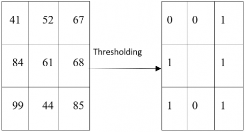
Another method tested in our work is involved in linear binary pattern (LBP) [17]. The local binary pattern was first introduced as a descriptor of the non-sensing pattern for the gray spectrum images. This operator produces a binary number for each pixel according to the label of neighboring 3x3 pixels. Labels are obtained by thresholding the value of neighboring pixels to the central pixel value. It is set for pixels with values greater than or equal to the central pixel value of label 1 and the pixels with values smaller than the central pixel value. It is set for pixels with values greater than or equal to the central pixel value of label 1 and the pixels with values smaller than the central pixel value of 0. These labels are then rotated to form an 8-bit number (Figure 5). This was done by just the central assessment and stipulating binary numbers for its neighbours. In our proposed system, we used uniform LBP to extract the feature of leaves.
Figure 5. LBP operator
4.2.3 Color features
This section is concerned with extraction of color features. It is done due to the features extraction in RGB color space is more effective than other color spaces. These statistical features are composed of mean (μ), standard deviation (σ), skewness (θ), and kurtosis (γ). Based on these statistical calculations, each plane of R, G, and B components consists of four features. The four statistical formulas can be defined as follows [18, 19]:
$\mu=\frac{1}{M N} \sum_{i=1}^{M} \sum_{j=1}^{N} p_{i j}$ (6)
$\sigma^{2}=\sqrt{\frac{1}{M N} \sum_{i=1}^{M} \sum_{j=1}^{N}\left(p_{i j}-\mu\right)^{2}}$ (7)
$\theta=\frac{\sum_{i=1}^{M} \sum_{j=1}^{N}\left(p_{i j}-\mu\right)^{3}}{M N \sigma^{3}}$ (8)
$\gamma=\frac{\sum_{i=1}^{M} \sum_{j=1}^{N}\left(p_{i j}-\mu\right)^{4}}{M N \sigma^{4}}-3$ (9)
where, M and N are dealt with the dimension of image, pij is the value of color on row j and column i.
4.3 Post processing phase
4.3.1 Feature normalization
In normalization process, we can map data from its current interval to another interval. This approach can be a great help for our forecasting and analytical purposes. There are a vast variety of forecasting models. To maintain this diversity, normalization techniques can help us to bring these forecasts closer together [7].
In the absence of normalization, features with large values lead to a stronger influence on the cost function in designing the classifier. Normalization can be conducted by using Eq. (10).
$\hat{x}=\frac{x_{i}-x_{\min }}{x_{\max }-x_{\min }}$ (10)
In this case, $\hat{x}$ represents new value of the feature, $\boldsymbol{x}_{i}$ describes primary value of the feature, $x_{m i n}$ is considered as the smallest value for primary feature and $x_{m a x}$ is considered as the largest value for primary feature.
4.3.2 Feature selection using PBPSO algorithm
Feature selection is taken into account as one of the most important steps in the data mining process. Therefore, a new Pbest-guide binary particle swarm optimization (PBPSO) is proposed to enhance the performance of BPSO [20]. In PBPSO, the velocity of a particle is updated in accordance with Eq. (11):
$v_{i}^{l+1}=w v_{i}^{l}+c_{1} r_{1}\left(\text { pbest }_{i}^{l}-\mathrm{X}_{i}^{l}\right)$
$+c_{2} r_{2}\left(\text { gbest }_{i}^{l}-\mathrm{X}_{i}^{l}\right)$ (11)
In Eq. (11), v signifies velocity; w denotes the inertia weight; c1 and c2 are cognitive and social learning vectors, respectively; r1 and r2 are two independent random vectors in [0,1]; X is the solution; pbest is the personal best solution; gbest is the global best solution for the whole population; l is the number of iterations; and d is the dimension of the search space.
At this point, the modified sigmoid function is used to convert the velocity to the probability. Eq. (12) represents this procedure.
$\mathrm{T}\left(\mathrm{v}_{\mathrm{i}}^{\mathrm{l}+1}\right)=\frac{1}{1+\exp (-10(0.5))}$ (12)
Now, update the new position of a particle through Eq. (13).
$\mathrm{x}_{\mathrm{i}}^{\mathrm{l}+1}=\left\{\begin{array}{c}1, \text { if } \mathrm{T} \mathrm{v}_{\mathrm{i}}^{\mathrm{l}+1}>\mathrm{r}_{0} \\ 0, \text { otherwise }\end{array}\right.$ (13)
where, $\mathrm{r}_{0}$ is a random vector in the interval of [0,1].
In the BPSO method, the position of pbest $_{i}$ Will be updated, if the fitness value of the new particle $X_{i}$ is larger than previous one. This updating mechanism can be calculated by Eq. (14).
pbest $_{i}^{1+1}=\left\{\begin{array}{c}\mathrm{x}_{i}^{1+1}, \text { if } \mathrm{f} \mathrm{x}_{\mathrm{i}}^{1+1}>\mathrm{F}\left(\text { pbest }_{i}^{1}\right) \\ \text { pbest }_{i}^{1}, \text { otherwise }\end{array}\right.$ (14)
In Eq. (14), F(.) is the fitness function, t denotes the number of iterations, X and pbest are dealt with the solution and personal best solution at the order of i in the population, respectively. Also, the pbest becomes, or approximately is the same as gbest. In this approach, crossover, mutation, and selection operators were considered for optimization process. There was an additional parameter, which is introduced as crossover rate (CR). This parameter needed tuning because the crossover operator was used for implementing and adjustment of the PBPSO algorithm. Crossover rate is computed by Eq. (15).
$C R=0.9-0.9\left(\frac{t}{T_{\max }}\right)$ (15)
In the Eq. (15), $T_{\max }$ is the maximum number of iterations and t is the number of iteration. Let f be a features dataset with I × D matrix, where I is the number of instances and D is the number of features. For feature selection, our goal was to achieve m features from the features dataset, where m<D. A summary of the feature selection process in PBPSO is shown in Figure 6.
4.3.3 Classification
The last step is coincided with classification of outcome feature vectors according to those species in which they belong. We have tested a total number of 4 classifiers. The best model is obtained through application of SVM classifier with quadratic kernel.
Decision Tree. A decision tree is a structure that is used to divide a large set of data into smaller chains of data. It is performed based on a set of simple decision rules. In each successive division, the members of the resulting sets are more or less similar to each other. This cluster is formed to categorize a large and heterogeneous population into smaller and more homogeneous groups with respect to a specific target variable [21].
k-Nearest Neighbors (k-NN). The k-Nearest Neighbors is considered as a nonparametric approach, which is used in data mining, machine learning, and pattern recognition. Here, the symbol "k" is characterized as a static value, and it often takes an odd value like 3, 5 ,7 and 9. Euclidean distance formula is used for measurment of distances between two entities and serves as a similarity index [15]. For instance, we have chosen 3 for the value of K. This value has been selected after testing few other values such as 5 and 7, but selection of 3 provided better results.
SVM. SVM is a binary classifier, which categorizes data into two classes. When the problem of classification requires more than two classes, just like our method for plant recognition, then multi-class SVM is used [10].
Naive Bayes. Simple Bayes classifier in machine learning is a group of probability-based simple classifiers that is applied together with simple independent random variables, assumed between different states and it is based on the Bayesian theorem. The Bayesian method is simply a kind of method for classifying phenomena based on the probability of occurrence or non-occurrence of a phenomenon [22].
In the proposed method, 5-fold cross-validation method is considered for 5 classifiers. In the 5-fold cross-validation method, if we randomly split the training dataset into k subsamples or layers with the same size, we can assign k-1 to each of these layers as the training dataset and one is used for the test dataset. The dataset was validated.
Figure 6. Flowchart of PBPSO for feature selection [20]
To implement and test the proposed method, a computer system has been employed for conducting the analysis processes. The computer system includes the following specifications: Windows 10, 64-bit, Intel Core i7-4720 CPU @ 2.60 GHz, 8 GB memory, and MATLAB R2018a. We analyzed the proposed method with respect to the accuracy,
precision, and recall. The accuracy of the proposed plant recognition system has been computed via the following expression, which utilizes the numerical details encompassing True Positive (TP) (it is the number of leaf images that have been correctly identified), False Positive (FP) (it is a parameter for representation of the number of leaf that are incorrectly detected), True Negative (TN) (it is a parameter for representation of the number of leaf images that are correctly detected), and False Negative (FN) (it is parameter for representation of the number of leaf images that are correctly recognized) [23].
Accuracy$=\frac{T P+T N}{N}$ (16)
Also, the precision and recall are defined as a measure for system evaluation. These concepts are calculated by Eqns. (17) and (18), respectively:
Precision $=\frac{T P}{T P+F P}$ (17)
Recall $=\frac{T P}{T P+F N}$ (18)
Further experiments were conducted to assess the effect of increasing the number of plant species and the number of leaves on the classification accuracy. The results are indicated in Figure 7 and Figure 8.However, the proposed plant identification system was tested on the Flavia dataset, which is included in leaf images of 32 plant species with 1600 samples [14]. Then, we tested the proposed method through Folio dataset that includes 640 leaves belonging to 32 different species of plants. We have applied 5-fold cross-validation without holdout. In each class, whole of the samples is decomposed into the tranining dataset (80%) and test dataset (20%). Description of Flavia Leaf dataset is shown in Table 1.
Table 1. Details description of Flavia leaf dataset
|
Scientific Name |
Name Common Name(s) |
Testing Sample |
|
Phyllostachys edulis (Carr.) Houz |
Pubescent Bamboo |
50 |
|
Aesculus chinensis |
Chinese Horse Chestnut |
50 |
|
Berberis anhweiensis Ahrendt |
Anhui Barberry |
50 |
|
Cercis chinensis |
Chinese Redbud |
50 |
|
Indigofera tinctoria L. |
True Indigo |
50 |
|
Phoebe nanmu (Oliv.) Gamble |
Nanmu |
50 |
|
Kalopanax septemlobus (Thunb. ex A.Murr.) |
Koidz. Castor Aralia |
50 |
|
Cinnamomum japonicum Sieb. |
Chinese Cinnamon |
50 |
|
Koelreuteria paniculata Laxm. |
Golden Rain Tree |
50 |
|
Ilex macrocarpa Oliv. |
Big-fruited Holly |
50 |
|
Pittosporum tobira (Thunb.) Ait. |
f. Japanese Cheesewood |
50 |
|
Chimonanthus praecox L. |
Wintersweet |
50 |
|
Cinnamomum camphora (L.) |
J. Presl Camphortree |
50 |
|
Viburnum awabuki K.Koch |
Japanese Arrowwood |
50 |
|
Osmanthus fragrans Lour. |
Sweet Osmanthus |
50 |
|
Cedrus deodara (Roxb.) G. |
Don Deodar |
50 |
|
Ginkgo biloba L. |
Ginkgo, Maidenhair Tree |
50 |
|
Lagerstroemia indica (L.) Pers. |
Crape myrtle, Crepe myrtle |
50 |
|
Nerium oleander L. |
Oleander |
50 |
|
Podocarpus macrophyllus (Thunb.) |
Sweet Yew Plum Pine |
50 |
|
Prunus serrulata Lindl. var. lannesiana auct. |
Japanese Flowering Cherry |
50 |
|
Ligustrum lucidum Ait. f. |
Glossy Privet |
50 |
|
Tonna sinensis M. Roem. |
Chinese Toon |
50 |
|
Prunus persica (L.) |
Batsch Peach |
50 |
|
Manglietia fordiana Oliv. |
Ford Woodlotus |
50 |
|
Acer buergerianum Miq. |
Trident Maple |
50 |
|
Mahonia bealei (Fortune) Carr. |
Beale’s Barberry |
50 |
|
Magnolia grandiflora L. |
Southern Magnolia |
50 |
|
Populus × Canadensis Moench |
Canadian Poplar |
50 |
|
Liriodendron Chinese (Hemsl.) Sarg. |
Chinese Tulip Tree |
50 |
|
Citrus reticulata Blanco |
Tangerine |
50 |
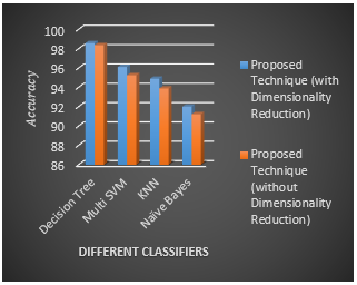
Figure 7. Comparison of the proposed approach with different classifiers using Flavia dataset
Figure 8. Comparison of the proposed approach with different classifiers using Folio dataset
According to the Figure 7, it can be noted that the tree classification provides the highest accuracy in comparison with the other methods. The accuracy of the tree classification is determined 98.58 and 98.37 with and without dimensionality, respectively. Also, according to the Figure 8, it can be found that the tree classification provides the highest accuracy in comparison with the other mentioned methods. The accuracy of the tree classification is ascertained 90.02 and 89.50 with and without dimensionality reduction, respectively. Table 2 and Table 2 and Table 3 represent the average percentage of accuracy and recall for different methods on the Flavia and Folio databases, respectively.
Table 2. Summary of the classification results and comparison of the proposed approach with different classifiers via Flavia dataset
|
Technique |
Flavia Dataset |
|
|
|
Proposed Technique (with Dimensionality Reduction) |
Classifier |
Accuracy |
Recall |
|
Decision Tree |
98.58% |
100% |
|
|
Multi SVM` |
96.12% |
98.06% |
|
|
KNN |
94.89% |
96.23% |
|
|
Naïve Bayes |
92.01% |
94.14% |
|
|
Proposed Technique (without Dimensionality Reduction) |
Decision Tree |
98.37% |
99.64% |
|
Multi SVM` |
95.25% |
96.34% |
|
|
KNN |
93.89% |
94.49% |
|
|
Naïve Bayes |
91.23% |
93.16% |
|
Table 3. Summary of the classification results and comparison of the proposed approach with different classifiers via Folio dataset
|
Technique |
Folio Dataset |
|
|
|
Proposed Technique (with Dimensionality Reduction) |
Classifier |
Accuracy |
Recall |
|
Decision Tree |
90.02% |
91.99 |
|
|
Multi SVM` |
88.02% |
90.3% |
|
|
KNN |
89.21% |
91.47% |
|
|
Naïve Bayes |
80.11% |
82.00% |
|
|
Proposed Technique (without Dimensionality Reduction) |
Decision Tree |
89.5% |
91.56% |
|
Multi SVM` |
87.11% |
89.65% |
|
|
KNN |
88.3% |
90.78% |
|
|
Naïve Bayes |
81.3% |
83.41% |
|
Table 2 and Table 3 give the average percentage of accuracy for different methods on the Flavia and Folio databases, respectively. Comparisons between Flavia and Folio databases indicate that our proposed algorithm provides the highest accuracy and Recall for the decision tree classifier among the other listed Classifiers.
Also, further experiments were conducted to assess the effect of increasing the number of features on the classification accuracy and recall. The results are displayed in Figure 9 and Figure 10.
According to the Figures 9 and 10, it can be noted that when the number of features is increased, then the accuracy enhances, as well. The gist features have considerable impact on the accuracy in comparison with the other features. One of the basic reasons that the proposed method performs better than other methods is dealt with application of the most comprehensive leaf features for extracting leaf features. Also, another possible reason refers to the gist properties that they are suitable for the same types. The proposed technique provides the accuracy of 98.58%, 93.89% and 91.23% through application of decision tree, KNN and Naïve Bayes, respectively. These results reveal that application of decision tree shows the best accuracy among the other methods. The differences occur in terms of their processing speed. For example, the decision tree is the fastest method.
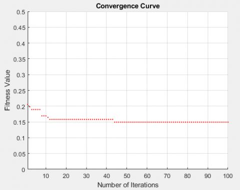
By implementing the PBPSO algorithm, the best fitness function was obtained at 100th iterations. This procedure is shown in Figure 10.
The best e fitness function used by Algorithm PBPSO was obtained at iteration 100 as shown in Figure 11.
Figure 9. Effect of increasing the number of different features on the accuracy of Flavia dataset
Figure 10. Effect of increasing the number of different features on the accuracy of Folio dataset
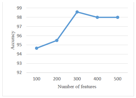
As shown in the Figure 10, the fitness function converges when the number of iterations increases to reach the interval of 50 and 100. This convergency procedure occurs through development of PBPSO algorithm in the feature selection process. By increasing the number of duplicates, it can be seen that the convergence is 0.15 in the repetition of 100. It indicates a very good performance reduction through development of PBPSO. The effects of PBPSO feature reduction performance on the Flavia and Folio datasets are depicted in Figures 12 and 13 below.
Figure 11. Fitness plot for Pbest-guide binary particle swarm optimization algorithm (PBPSO)
Figure 12. Effects of the performance of PBPSO feature reduction method on Flavia dataset
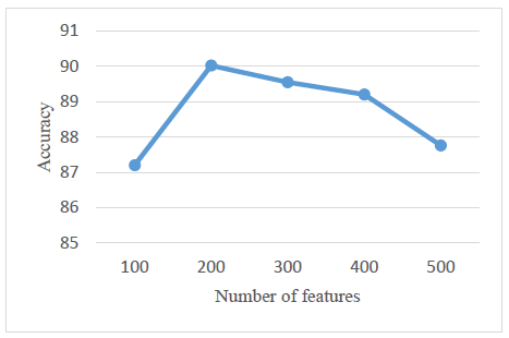
Figure 13. Effects of the performance of PBPSO feature reduction method on Folio dataset
As can be seen in Figure 12, this method works best when the number of features reaches 300.
Figure 12 and Figure 13 show the performance of different features using the PBPSO method on the Folio dataset. When the number of features reaches about 200, the best classification performance is achieved.
Tables 4 and 5 represent the average percentage of accuracy for both the prevalent existing methods and the proposed method on the Flavia and Folio databases, respectively.
Comparisons between Flavia and Folio databases indicate that our proposed algorithm has the highest accuracy and sensitivity in comparison with the other listed methods.
Given the wide variety of features extracted from images, it is obvious that the image processing stage requires a longer time. Therefore, Tables 6 and 7 compare the performance of time complexity in seconds based on different classifications to classify training and test features.
Table 4. Comparison of the proposed technique with the existing prevalent approaches using Flavia dataset
|
Technique |
Flavia Dataset |
|
|
Classifier |
Accuracy |
|
|
Wu et al. (2007b) [2] |
PNN |
90.3% |
|
Krishna et al. (2010) [10] |
PNN |
91% |
|
Arun Priya et al. (2012) [1] |
KNN, SVM |
94.5% |
|
Gwo and Wei (2013) [11] |
Bayesian |
92.7% |
|
Satti et al. (2013) [13] |
ANN |
93.3% |
|
Kadir et al. (2013) [3] |
PNN |
93.75% |
|
Lavania and Matey (2014)[14] |
SIFT |
87.5% |
|
Aakif and Khan [6] |
ANN |
96% |
|
Proposed Technique |
Decision Tree |
98.58 |
Table 5. Comparison of the proposed technique with the existing prevalent approaches using Folio dataset
|
Technique |
Folio Dataset |
|
|
Classifier |
Accuracy |
|
|
Munisamia et al. [9] |
KNN |
87.2% |
|
Proposed Technique |
Decision Tree |
90.02 |
|
Classifier |
Training time per classification [sec] |
|
KNN |
1.485 |
|
Naïve Bayes |
3.890 |
|
Multi SVM` |
8.568 |
|
Decision Tree |
2.036 |
Table 7. Comparison of the testing time of the classifiers using the proposed technique
|
Classifier |
Testing time per classification [sec] |
|
KNN |
0.485 |
|
Naïve Bayes |
1.243 |
|
Multi SVM` |
3.022 |
|
Decision Tree |
0.687 |
Tables 5 and 6, present the mean classification time, which is considered with respect to datasets Folio and Flavia.
In this paper, we presented a novel technique to detect plant leaf images by combining Shape, color, vein, gist and LBP features, and then classify the leaves using decision tree.
An important point refers to the feature extraction and classification of leaves with congested and uneven edges. In many of the previous algorithms, processing of these types of images is dealt with a significant computational complexity. However, the proposed method has the ability to simply process these types of images using gist features vector. The proposed method provides the accuracy of above 95%.
We carried out our experiment on a publicly available dataset, called Flavia and Folio Leaf Datasets. Then, a new feature reduction method (i.e. Pbest-guide binary particle swarm optimization (PBPSO)) is presented to enhance the performance of BPSO. The performance analysis shows that the proposed system offers higher accuracy than the existing prevalent techniques. Classifiers show different accuracies in comparison with each other. Decision tree works better than the other methods for leaf identification. According to these results, recognition performance, the decision tree method has obtained the accuracy of 98.58% and 90.02 on Flavia and Folio leaf datasets, respectively. The experiment shows the effectiveness of the most comprehensive set of leaf parameters for extraction of the best discriminatory features over plant leaves detection.
[1] Priya, C.A., Balasaravanan, T., Thanamani, A.S. (2012). An efficient leaf recognition algorithm for plant classification using support vector machine. In International Conference on Pattern Recognition, Informatics and Medical Engineering (PRIME-2012), pp. 428-432. https://doi.org/10.1109/ICPRIME.2012.6208384
[2] Wu, S.G., Bao, F.S., Xu, E.Y., Wang, Y.X., Chang, Y.F., Xiang, Q.L. (2007). A leaf recognition algorithm for plant classification using probabilistic neural network. In 2007 IEEE International Symposium on Signal Processing and Information Technology, pp. 11-16. https://doi.org/10.1109/ISSPIT.2007.4458016
[3] Kadir, A., Nugroho, L.E., Susanto, A., Santosa, P.I. (2013). Leaf classification using shape, color, and texture features. arXiv preprint arXiv:1401.4447. 225-230, Computer Vision and Pattern Recognition.
[4] Zheng, X.D., Wang, X.J. (2009). Feature extraction of plant leaf based on visual consistency. In 2009 International Symposium on Computer Network and Multimedia Technology, pp. 1-4. https://doi.org/10.1109/CNMT.2009.5374826
[5] Bhardwaj, A., Kaur, M., Kumar, A. (2013). Recognition of plants by leaf image using moment invariant and texture analysis. International Journal of Innovation and Applied Studies, 3(1): 237-248.
[6] Aakif, A., Khan, M.F. (2015). Automatic classification of plants based on their leaves. Biosystems Engineering, 139: 66-75. https://doi.org/10.1016/j.biosystemseng.2015.08.003
[7] Choras, R.S. (2007). Image feature extraction techniques and their applications for CBIR and biometrics systems. International Journal of Biology and Biomedical Engineering, 1(1): 6-16.
[8] Acharya, T., Ray, A.K. (2005). Image Processing Principles and Applications. John Wiley & Sons.
[9] Munisam, T., Ramsurn, M., Kishnah, S., Pudaruth, S. (2015). Plant leaf recognition using shape features and colour histogram with K-nearset neighbour classifiers. Procedia Computer Science, 58: 740-747.
[10] Singh, K., Gupta, I., Gupta, S. (2010). SVM-BDT PNN and Fourier moment technique for classification of leaf shape. International journal of signal processing. Image Processing and Pattern Recognition, 3(4): 67-78.
[11] Gwo, C.Y., Wei, C.H. (2013). Plant identification through images: using feature extraction of key points on leaf contours. Applications in Plant Sciences, 1(11): 1200005. https://doi.org/10.3732/apps.1200005
[12] Islam, M.A., Yousuf, M.S.I., Billah, M.M. (2019). Automatic plant detection using HOG and LBP features with SVM. International Journal of Computer (IJC), 33(1): 26-38.
[13] Satti, V., Satya, A., Sharma, S. (2013). An automatic leaf recognition system for plant identification using machine vision technology. International Journal of Engineering Science and Technology, 5(4): 874.
[14] Lavania, S., Matey, P.S. (2014). Leaf recognition using contour based edge detection and SIFT algorithm. In 2014 IEEE International Conference on Computational Intelligence and Computing Research, pp. 1-4. https://doi.org/10.1109/ICCIC.2014.7238345
[15] Saleem, G., Akhtar, M., Ahmed, N., Qureshi, W.S. (2019). Automated analysis of visual leaf shape features for plant classification. Computers and Electronics in Agriculture, 157: 270-280. https://doi.org/10.1016/j.compag.2018.12.038
[16] Kheirkhah, F.M., Asghari, H. (2018). Plant leaf classification using GIST texture features. IET Computer Vision, 13(4): 369-375. https://doi.org/10.1049/iet-cvi.2018.5028
[17] Ojala, T., Pietikäinen, M., Harwood, D. (1996). A comparative study of texture measures with classification based on featured distributions. Pattern Recognition, 29(1): 51-59. https://doi.org/10.1016/0031-3203(95)00067-4
[18] Iwata, T., Saitoh, T. (2013). Tree recognition based on leaf images. In The SICE Annual Conference 2013, pp. 2489-2494.
[19] Kadir, A., Nugroho, L.E., Susanto, A., Santosa, P.I. (2012). Experiments of Zernike moments for leaf identification. Journal of Theoretical and Applied Information Technology (JATIT), 41(1): 82-93. https://repository.ugm.ac.id/id/eprint/36075
[20] Too, J., Abdullah, A.R., Mohd Saad, N., Tee, W. (2019). EMG feature selection and classification using a Pbest-guide binary particle swarm optimization. Computation, 7(1): 12. https://doi.org/10.3390/computation7010012
[21] Fayyad, U.M., Irani, K.B. (1992). On the handling of continuous-valued attributes in decision tree generation. Machine Learning, 8(1): 87-102. https://doi.org/10.1007/BF00994007
[22] Lewis, D.D. (1998). Naive (Bayes) at forty: The independence assumption in information retrieval. In European Conference on Machine Learning, 1398: 4-15.
[23] Vijaya Lakshmi, B., Mohan, V. (2016). Kernel-based PSO and FRVM: An automatic plant leaf type detection using texture, shape, and color features. Computers and Electronics in Agriculture, 125: 99-112. https://doi.org/10.1016/j.compag.2016.04.033