Weili Meng* | Chuanzhong Mao | Jin Zhang | Jing Wen | Dehua Wu
© 2019 IIETA. This article is published by IIETA and is licensed under the CC BY 4.0 license (http://creativecommons.org/licenses/by/4.0/).
OPEN ACCESS
In recent years, a massive number of images have generated on the online social network (OSN). This calls for an efficient and rapid way to extract the information from the OSN images. This paper puts forward an OSN image classification method based on improved deep belief network (DBN) and support vector machine (SVM). In the proposed method, the image classification is enhanced by improving the self-adaptive learning rate based on incremental discrimination of reconstruction error and the weight update criteria with increasing momentum. The effectiveness of our method was confirmed through an image recognition experiment on OSN images obtained from Sina Weibo public platform, in comparison with four commonly used classification methods. The research results shed new light on feature extraction and classification of OSN images.
online social network (OSN), image recognition, deep learning, image classification, support vector machine (SVM)
In the era of the Internet, online social network (OSN) has permeated deeply into our daily life. The OSN allows users to exchange and share information anytime and anywhere. The ubiquitous information exchange leads to an exponential growth of the OSN data [1]. As an important part of OSN data, images carry lots of important information. However, the surging number of images in the OSN poses a severe challenge to organized image storage. In fact, it is increasingly difficult to find the desired image out of the massive number of images. What is worse, the rich information contained in the OSN images has not been effectively utilized. In image processing, it is a research hotspot to classify the OSN images and extract information from them in a quick and accurate manner.
By the design principle of image classifier, the common image classification methods can be divided into two categories: those based on production model [2], and those based on discriminant model [3]. The former statistically represents the data distribution and reflects the similarity between images, in the light of the joint probability distribution of image features and classes. The latter identifies the differences between image classes and finds the optimal classification surface between them, according to the conditional probability distribution of image features and classes. The typical methods based on production model include Bayesian classification model [4] and Gaussian mixture model [5], and the most representative methods based on discriminant model include nearest neighbor method [6], decision tree [7] and artificial neural network (ANN) [8]. Both types of image classification methods face the defects of being shallow classification techniques. For example, the features cannot be expressed well if the training sample is insufficient or the data dimension is too large.
The above defects can be solved by the machine learning technique of deep learning, which extracts sample features and recognizes and classifies patterns through supervised or unsupervised learning, using multilayer nonlinear deep network structure. Mimicking the hierarchical structure of visual neural system, deep learning can extract the input data iteratively, mine the high-level features out of the data, and thus enhance the classification or prediction performance.
This paper applies the deep learning model to mine out the information in OSN image samples, aiming to achieve fast and accurate image recognition.
Image classification [9] generally relies on computer technology to automatically obtain the semantic information of image features, and divide the information into preset classes based on the image content. For example, Li et al. [10] proposed a hybrid feature selection strategy based on support vector machine (SVM) and genetic algorithm (GA), and classified hyperspectral remote sensing images by the strategy. Liang et al. [11] put forward an image classification method based on convolutional neural network (CNN). Han et al. [12] presented a multi-label image classification algorithm based on neural network (NN). Smitha et al. [13] optimized the weights of backpropagation neural network (BPNN) with conjugate gradient algorithm, and applied the weight optimization method to classify magnetic resonance imaging (MRI) brain images. Zhang et al. [14] found that the SVM performs poorly in classifying a small number of unbalanced samples, improved the SVM algorithm and adopted the improved version for medical image classification. Xu et al. [15] proposed a nonnegative constrained local linear coding method for image classification, which achieves excellent classification effect.
Deep learning can classify largescale samples both accurately and efficiently, and has been widely used in image classification. For instance, Cheng et al. [16] successfully employed deep learning to classify remote sensing images. Zhao et al. [17] designed a deep convolutional coder for the classification of high-resolution synthetic-aperture radar (SAR) images, which is immune to the speckle noise in these images. Liu et al. [18] developed a discriminative deep belief network (DBN) for image classification. Lunga et al. [19] created a hybrid deep learning network for image classification, in which high-level features are extracted by a sparse automatic encoder and then the images are classified by the DBN. Ejbali et al. [20] combined wavelet network and deep learning into a deep convolutional wavelet network for image classification. Zhang et al. [21] proposed a training method of DBN model with a distributed parallel computing framework.
Despite its immense popularity in image classification, deep learning faces three prominent problems. First, the deep learning model is prone to overfitting and the local minimum trap in the training process. Second, the deep learning model often has a complex structure with multiple parameters, and requires iterative calculation in the training process, both of which push up the computing load. Third, there is no general deep learning model for image classification, although many models have been adopted individually.
3.1 DBN
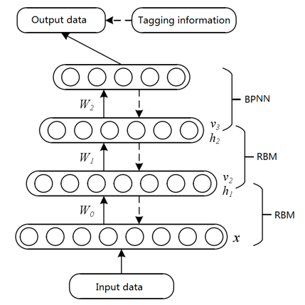
The DBN [22] is a deep learning model commonly used in image classification. As shown in Figure 1, the DBN typically consists of multiple layers of restricted Boltzmann machines (RBMs) and one layer of supervised BPNN [23].
Figure 1. Structure of the DBN
The training process of the DBN model usually covers two phases: pretraining and finetuning. In the pretraining phase, the RBM layers are trained from bottom to top by greedy unsupervised learning algorithm. Only one layer of the RBM is trained at a time, such that the feature vector can retain as much feature information as possible before mapping to different feature spaces. In the finetuning phase, the RBM output is taken as the input of the BPNN superimposed on the top layer of the DBN, and the DBN parameters are finetuned from top to bottom through traditional supervised learning [24].
The RBM, the basic structure of the DBN model, serves as the basic unit of DBN training. Hinton et al. proposed the CD-k algorithm [25], which reduces the large sampling steps facing the high dimension of training sample data. However, there are still problems with the selection of the initial learning rate in the pretraining phase. During the CD-k-based RBM training, the network is usually trained by a small global learning rate. If the learning rate is too high, the reconstruction error will increase sharply, making the algorithm unstable and fall into the local minimum. If the learning rate is too small, the instability and local minimum trap will be avoided, but the convergence will slow down and the training time will become excessively long. Therefore, it is crucial to choose a suitable learning rate for the DBN training.
In this paper, the DBN is trained at a changing learning rate instead of a global learning rate. To speed up the convergence, the momentum term was added to the update criteria of connection weight $W_{i j}$ and biases $a_{i}$ and $b_{j}$ . In this way, the weight and bias terms after the n-th iteration partially depend on the updated value after the (n-1)-th iteration.
3.2 Improved DBN training algorithm
The first step to improve the DBN training is to set a suitable initial learning rate $\sigma$ for the RBM training algorithm. If the reconstruction error increases after one iteration, then the initial learning rate is too large, and should be reduced by multiplying it with a constant less than 1. Otherwise, this iteration is effective, and the learning rate should be kept for the next iteration. The iterative process should be terminated, once the learning rate falls below the specified minimum.
The improved RBM training algorithm can automatically adjust the learning rate $\delta_{i j}$ , rather than use a fixed learning rate $\sigma$ in the DBN. This self-adaptive learning rate $\delta_{i j}$ can be calculated by:
$\delta_{i j}^{\prime}=\left\{\begin{array}{ll}
{\delta_{i j},} & {\text { if } \Delta e_{n}>0} \\
{\varphi \times \delta_{i j},} & {\text { if } \Delta e_{n}<0}
\end{array}\right.$ (1)
where, $\varphi \in[0,1]$ is the decrement factor; $\Delta e_{n}=e_{n}-e_{n-1}$ , with $e_{n}$ and $e_{n-1}$ being the reconstruction errors after n iterations and n-1 iterations, respectively. If $\Delta e_{n}>0$ , then the reconstruction error increases after one iteration; if $\Delta e_{n}<0$ , then the reconstruction error decreases after one iteration.
As mentioned before, in the improved RBM training algorithm, a momentum term is added to the update criteria of connection weight $W_{i j}$ and biases $a_{i}$ and $b_{j}$ . In this way, the weight and bias terms after the n-th iteration partially depend on the updated value after the (n-1)-th iteration. The new update criteria make the update faster in the same direction, thereby speeding up the convergence and reducing the training time.
The self-adaptive learning rate and new update criteria were also applied to the DBN training algorithm. After training on each layer of the RBM, the learning rate should be updated according to Eq. (1). In the next training, the weight and biases should be updated according to the new update criteria.
The basic process of the improved RBM training algorithm is as follows:
|
Improved RBM training algorithm |
|
Input: Initial connection weight $W_{i j}$ , initial biases $\boldsymbol{a}_{\boldsymbol{i}}$ and $b_{j}$ , initial learning rate $\delta_{0}$ , number of iterations R, and minimum learning rate $\delta_{m i n}$ . Output: Connection weight W , biases $\boldsymbol{a}$ and b , and self-adaptive learning rate $\delta_{i j}^{n e w}$ . |
|
1. For r=1, 2,…, R ,. do 2. Calculate the random node states of visible layer and hidden layer of each RBM. 3. Calculate the likelihood gradient of weight and biases. 4. Calculate the likelihood gradient increment of weight and biases. 5. Calculate the reconstruction error $\Delta e_{n}, \Delta e_{n}=e_{n}-e_{n-1}$ . 6. Update weight $W_{i j}$ and biases $\boldsymbol{a}_{\boldsymbol{i}} \text { and } \boldsymbol{b}_{\boldsymbol{j}}$ , $W_{i j}^{\prime} \leftarrow W_{i j}+\Delta W_{i j}, a_{i}^{\prime} \leftarrow a_{i}+\Delta a_{i}, b_{j}^{\prime} \leftarrow b_{j}+\Delta b_{j}$ . 7. Adjust the self-adaptive learning rate $\boldsymbol{\delta}_{i j}^{\prime}$ based on the increment of reconstruction error, and take it as the learning rate of lower-layer RBM training. 8. End for |
As mentioned before, the training of the DBN covers the unsupervised pretraining and the supervised finetuning. In the improved DBN training algorithm, the DBN is constructed and trained layer-by-layer by the improved RBM training algorithm from the bottom to the top. After training, the weight and biases of each layer of RBM are outputted.
The basic process of the improved DBN training algorithm is as follows:
|
Improved DBN training algorithm |
|
Input: Training data set T , initial connection weight $W_{i j}$ , initial bias $\boldsymbol{a}_{i}$ and $b_{j}$ , initial learning rate $\delta_{0}$ , number of iterations R , and number of hidden layers H . Output: Weight and biases obtained through final training |
|
1. Pretraining phase: 2.For k=1,2,…, $H-1$ ,. do 3. For r=1,2,…, R ,. do 4. If k=1, then 5. Call improved RBM training algorithm, and save learned weight $W_{1}$ , biases $\boldsymbol{a}_{\mathbf{1}}$ and $b_{1}$ and learning rate $\boldsymbol{\delta}_{i j}^{1}$ . 6. else 7. Call improved RBM training algorithm, and save learned weight $W_{l}$ , biases $\boldsymbol{a}_{\boldsymbol{l}}$ and $b_{l}$ and learning rate $\boldsymbol{\delta}_{i j}^{l}$ . 8. End else 9. End for 10. End for 11. Finetuning phase: 12. Take the weight, biases and learning rate obtained after the pretraining of all the layers of RBMs as the inputs. 13. For r=1, 2,…, R ,. Do 14. Call the BPNN algorithm to calculate the spatial parameters of all RBM layers, including weight gradient and biases, and call the gradient descent algorithm to update weight gradient 15. End for |
3.3 Image classification method based on improved DBN
This paper employs the improved DBN to extract image features, and then classifies images by the SVM, a machine learning algorithm widely used for regression and classification problems (Figure 2).
The feature extraction was carried out in three steps. Firstly, feature vector of the preprocessed image was imported to the DBN. Next, the network was trained and constructed by the improved DBN training algorithm. Finally, the weight parameters of the network space were further optimized by the gradient descent algorithm, enabling the DBN network to extract the deep features of the input image layer by layer in the bottom-up direction. Once the DBN has been trained, the output of the last hidden layer was inputted to the SVM classifier, aiming to train the classifier and obtain the SVM parameters. After that, the trained DBN was applied to extract the features of image samples.
When it comes to image classification and recognition, the preprocessed image was input into the trained DBN as a feature vector, and processed by the SVM classifier after feature extraction.
Figure 2. Image classification based on improved DBN and the SVM
As shown in Figure 2, the main difference of the DBN-based classification method from the traditional method lies in its uniqueness of feature extraction. In the traditional method, the image features are often extracted by an artificial structure algorithm. In the DBN-based method, the features of the input image are extracted automatically layer-by-layer from the bottom by a deep learning model with multiple hidden layers.
The OSN images contain much more information than ordinary images, such as the geographic location and time. If the information can be extracted quickly and effectively, the images will be classified much more easily.
There are two basic ways to retrieve images: text-based method and content-based method. The former method mainly transforms image retrieval into the keyword retrieval. The keywords are marked manually according to the subject, source, author or size of the image, such that the image can be retrieved based on the keywords. The latter method mainly utilizes on the similarity between the feature vector of the image to be retrieved and the feature vector of the image in the image library. Computer technology is introduced to automatically extract color features, shape features, texture features or higher-level features of the image, and then the similarity matching algorithm is adopted to retrieve the image.
The two methods have similar retrieval processes: image preprocessing, feature (keyword) extraction, similarity matching, and result output. The image retrieval bears high resemblance with image classification. The core of both processes is feature extraction. Through image retrieval, the text information like image keywords can be defined as the text features of image, and the features of image color, shape and texture or higher-level features that reflect the internal attributes of image can be defined as the content features of image.
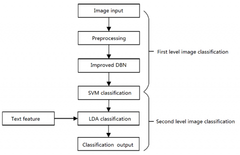
Figure 3. The two-level OSN image recognition algorithm
In addition to the OSN image, the authors also saved the geographic location, creation time and other text information of the image. Therefore, the image features obtained by the deep learning model and the text information of the OSN image were attributed to the content features and the text features of the image, respectively.
Compared with ordinary images, the OSN images have two unique attributes, namely, geographic location and creation time. Here, the two attributes are treated as two dimensions of feature vector. Then, the classification of the OSN images was divided into two levels. In the first level, the image classification method based on improved DBN was directly used to handle the preprocessed OSN image feature vector. In the second level, the linear discriminant analysis (LDA) [26] was performed to classify the results of the first level based on time interval and geographic location. The two-level OSN image recognition algorithm is illustrated in Figure 3.
As shown in Figure 3, the proposed OSN image recognition method is essentially a multi-label classification method, which improves the efficiency of text feature extraction.
To verify its effectiveness, the proposed algorithm was applied to recognize the OSN images obtained by the application program of Sina Weibo open platform. The images contain various information, such as geographic location, creation time, city code and other text information.
Before the image recognition, the images obtained from Sina Weibo were screened, leaving only those on six luxury brands (Figure 4). The attention of these brands in different regions and periods of time was also discussed to improve the promotional activities on e-commerce platforms.
Figure 4. The luxury brands selected for our experiment
The images obtained from Sina Weibo are all shot and uploaded manually. Many of them are severely distorted and unclear, adding to the difficulty of recognition. Hence, some clear images on luxury brand were added to the training set, which also comes from OSNs.
The final training set consists of 3,600 images, including 600 images on each brand. The test set also encompasses the images on the six brands, all of which are from Sina Weibo open platform. There is a total of 900 images in the test set, but the number of images varies from brand to brand. All the images were preprocessed by aggregation and normalization, and the preprocessed images are of the size 32×32 pixels.
Because the number of input layer nodes must equal the dimension of the feature vector of the image input, the number of these nodes was set to 1,024. Meanwhile, the number of output layer nodes was set to 6, because it should equal the number of classes of the data samples.
The image recognition is greatly affected by the depth of the DBN and the number of iterations. Therefore, our experiment focuses on how the number of hidden layers and the number of iterations influence the recognition performance, aiming to optimize the network structure based on experimental data.
In our experiment, the number of random nodes in input, output and hidden layers was set to 700, 10 and 400, respectively. The learning rate and biases were initialized as 0.1 and 0, respectively. The connection weight was randomly obtained from the Gaussian distribution with the mean of 0 and the standard deviation of 0.01. The number of hidden layers was set to 2,3,4,5 respectively, while the number of iterations was increased from 100 to 500, at the step length of 50. Only one combination of the number of hidden layers and that of iterations was tested at a time, to reveal how the two parameters affect the classification performance.
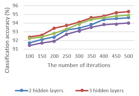
The classification accuracy of the OSN image recognition algorithm for different parameter combinations is presented in Figure 5.
Figure 5. The influence of different parameter combinations on classification performance
As shown in Figure 5, when the number of iterations remained the same, the number of hidden layers had an important impact on the accuracy of image classification. However, the classification accuracy was not necessarily increasing with the growing number of hidden layers. This means too many hidden layers may suppress the DBN’s generalization ability, thus undermining the classification performance.
When the number of hidden layers remained unchanged, the accuracy of image classification initially increased with the number of iterations. However, when the number of iterations exceeded 400, the improvement of classification accuracy was no longer obvious.
Therefore, the number of hidden layers DBN should be set to 3, and each hidden layer should contain 400 random nodes.
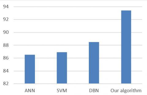
Furthermore, our algorithm, the improved DBN, was compared with the ANN, the SVM and the DBN image classification methods on the same dataset. The classification accuracy of different algorithms is shown in Figure 6.
Figure 6. Comparison of classification accuracy of different classification methods
It can be seen that the DBN outperformed the ANN and the SVM, revealing the strength of the DBN in feature extraction and the advantage of deep learning in image classification. Moreover, the improved DBN achieved better classification results than the DBN, an evidence of the effectiveness of our algorithm.
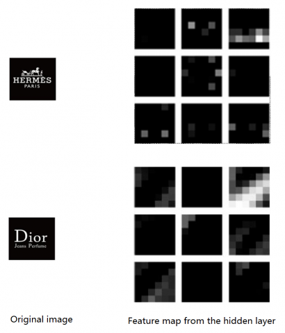
Finally, our algorithm was tested on two samples of OSN images. The feature maps learned from the images in the hidden layer are provided in Figure 7.
As shown in Figure 7, the contour of the feature maps generated by the hidden layer was unclear, indicating that the obtained images are very abstract. Like human vision system, our algorithm first extracts the edge features from the target images, obtains the initial shape features, abstracts high-level features, and recognizes the target in turn. This process reflects the deep learning principle: extracting the features of the input image from the low-level features to the high-level features.
Figure 7. Feature map of OSN image samples in hidden layer
This paper proposes a two-level recognition algorithm for the OSN images based on improved DBN and the SVM, and verifies the effectiveness and accuracy of the algorithm compared to the other commonly used image classification algorithms. Of course, this paper only extracts the features with the help of deep learning, failing to filter the extracted features. The future research will optimize the extracted features and improve classification performance.
This work is supported by Social Science Planning Research Project of Shandong Province (Grant No.: 17CYYZ01).
[1] Kaur, R., Singh, S., Kumar, H. (2018). AuthCom: Authorship verification and compromised account detection in online social networks using AHP-TOPSIS embedded profiling based technique. Expert Systems with Applications, 113: 397-414. https://doi.org/10.1016/j.eswa.2018.07.011.
[2] Lee, J.Y., Lim, J.W., Koh, E.J. (2018). A study of image classification using HMC method applying CNN ensemble in the infrared image. Journal of Electrical Engineering & Technology, 13(3): 1377-1382. https://doi.org/10.5370/JEET.2018.13.3.1377
[3] Kaur, T., Saini, B.S., Gupta, S. (2018). A novel feature selection method for brain tumor MR image classification based on the Fisher criterion and parameter-free Bat optimization. Neural Computing & Applications, 29(8): 193-206. https://doi.org/10.1007/s00521-017-2869-z
[4] Fang, Y., Xu, L.L., Peng, J.H., Yang, H.L., Wong, A., Clausi, D.A. (2018). Unsupervised Bayesian classification of a hyperspectral image based on the spectral mixture model and Markov random field. IEEE Journal of Selected Topics in Applied Earth Observations and Remote Sensing, 3325-3337. https://doi.org/10.1109/JSTARS.2018.2858008
[5] Huang, Z.K., Chau, K.W. (2008). A new image thresholding method based on Gaussian mixture model. Applied Mathematics and Computation, 205(2): 899-907. https://doi.org/10.1016/j.amc.2008.05.130
[6] Yue, J., Wang, Y.P., Li, Z.B., Zhang, Z.W., Hou, J.L. (2014). A new image retrieval method based on K-nearest neighbor multistage and multiple features. Sensor Letters, 12(3): 479-484(6). https://doi.org/10.1166/sl.2014.3154
[7] Liu, Y., Zhang, D.S., Lu, G.J. (2008). Region-based image retrieval with high-level semantics using decision tree learning. Pattern Recognition, 41(8): 2554-2570. https://doi.org/10.1016/j.patcog.2007.12.003
[8] Raju, P., Rao, V.M., Rao, B.P. (2018). Grey wolf optimization-based artificial neural network for classification of kidney images. Journal of Circuits Systems and Computers, 27(14): 1850231. https://doi.org/10.1142/S0218126618502316.
[9] Vidyarthi, A., Mittal, N. (2016). AVNM: A voting based novel mathematical rule for image classification. Computer Methods and Programs in Biomedicine, 137: 195-201. https://doi.org/10.1016/j.cmpb.2016.08.015
[10] Li, S.J., Wu, H., Wan, D.S., Zhu, J.L. (2011). An effective feature selection method for hyperspectral image classification based on genetic algorithm and support vector machine. Knowledge-Based Systems, 24(1): 40-48. https://doi.org/10.1016/j.knosys.2010.07.003
[11] Liang, T.M., Xu, X.Z., Xiao, P.C. (2017). A new image classification method based on modified condensed nearest neighbor and convolutional neural networks. Pattern Recognition Letters, 94: 105-111. https://doi.org/10.1016/j.patrec.2017.05.019
[12] Han, M., Zhu, X.R., Yao, W. (2012). Remote sensing image classification based on neural network ensemble algorithm. Neurocomputing, 78(1): 133-138. https://doi.org/10.1016/j.neucom.2011.04.044
[13] Smitha, J.C., Babu, S.S. (2014). MRI brain image classification using Haar wavelet and artificial neural network. Advances in Intelligent Systems and Computing, 325: 253-261. https://doi.org/10.1007/978-81-322-2135-7_28
[14] Zhang, L., Shao, Z.F. (2014). Hyperspectral remote sensing image classification based on improved OIF and SVM algorithm. Science of Surveying & Mapping, 9263(13): 92632P-92632P-7.
[15] Xu, W., Wu, S., Er, M.J., Zheng, C., Qiu, Y. (2017). New non-negative sparse feature learning approach for content-based image retrieval. IET Image Processing, 11(9): 724-733.
[16] Cheng, G., Yang, C., Yao, X., Guo, L., Han, J.W. (2019). When deep learning meets metric learning: Remote sensing image scene classification via learning discriminative CNNs. IEEE Transactions on Geoscience and Remote Sensing, 56(5): 2811-2821. https://doi.org/10.1109/TGRS.2017.2783902
[17] Zhao, Z.Q., Jiao, L.C., Hou, B., Wang, S., Zhao, J.Q., Chen, P.H. (2016). Locality-constraint discriminant feature learning for high-resolution SAR image classification. Neurocomputing, 207: 772-784. https://doi.org/10.1016/j.neucom.2016.05.065
[18] Liu, S., Bai, X. (2012). Discriminative features for image classification and retrieval. Pattern Recognition Letters, 33(6): 744-751. https://doi.org/10.1016/j.patrec.2011.12.008
[19] Lunga, D., Yang, H.L., Reith, A., Weaver, J., Yuan, J.Y., Bhaduri, B. (2018). Domain-adapted convolutional networks for satellite image classification: A large-scale interactive learning workflow. IEEE Journal of Selected Topics in Applied Earth Observations and Remote Sensing, 11(3): 962-977. https://doi.org/10.1109/JSTARS.2018.2795753
[20] Ejbali, R., Zaied, M. (2018). A dyadic multi-resolution deep convolutional neural wavelet network for image classification. Multimedia Tools and Applications, 77(5): 6149-6163. https://doi.org/10.1007/s11042-017-4523-2
[21] Zhang, Q.C., Yang. L.T., Chen, Z.K., Li, P. (2018). A survey on deep learning for big data. Information Fusion, 42: 146-157. https://doi.org/10.1016/j.inffus.2017.10.006
[22] Hinton, G.E. Salakhutdinov, S.S. (2006). Reducing the dimensionality of data with neural networks. Science, 313(5786): 504-507. https://doi.org/10.1126/science.1127647
[23] Bin, S., Sun, G., Chen, C.C. (2019). Analysis of functional brain network based on electroencephalography and complex network. Microsystem Technologies, 99: 1-9. https://doi.org/10.1007/s00542-019-04424-0
[24] Huang, S.L., Zheng, X.L., Chen D.R. (2013). A semi-supervised learning method for product named entity recognition. Journal of Beijing University of Posts and Telecommunications, 36(2): 20-113.
[25] Hinton, G.E., Osindero, S., The, Y.W. (2006). A fast learning algorithm for deep belief nets. Neural Computation, 18(7): 1527-1554. https://doi.org/10.1162/neco.2006.18.7.1527
[26] Chen, L.H., Jiang, C.R. (2018). Sensible functional linear discriminant analysis. Computational Statistics & Data Analysis, 126: 39-52. https://doi.org/10.1016/j.csda.2018.04.005