Mohammed Abdul Wajeed* | Vallamchetty Sreenivasulu
© 2019 IIETA. This article is published by IIETA and is licensed under the CC BY 4.0 license (http://creativecommons.org/licenses/by/4.0/).
OPEN ACCESS
The convolutional neural network (CNN) and other neural networks (NNs) provide promising tools for robotized characterization of tumor cells. However, the tumor growth areas in ultrasound images are normally obscure, with uncertain edges. It is not acceptable to prepare ultrasound images straightforwardly with the CNN. To solve the problem, this paper puts forward a faster region-convolutional neural network (R-CNN) to identify tumor cells with the aid of auto encoders. Taking two fully-connected layers with dropout and ReLU enactments as the base, the proposed faster R-CNN adopts 3D convolutional and max pooling layers, enabling the user to extract features from potential tumor growth areas. In addition, the thin and deep layers of the network were connected to facilitate the identification of blurry or small tumor growth areas. Experimental results show that the proposed faster R-CNN with auto encoders outperformed traditional data mining and artificial intelligence (AI) methods in prediction accuracy of tumor cells.
convolutional neural network, region- convolutional neural network, tumor cells, pre processing, clustering, classification, tumor prediction
Tumor cell arrangement is very important task in medical findings, customized treatment and tumor avoidance. However, clustering various kinds of tumor cells with high exactness has remained a difficult task and furthermore a few effects brought about by outer conditions. These can affect the precision of tumor cell clustering.
Luckily, AI has been growing quickly as a significant instrument for such troublesome task as of late, incorporating into the field of science and medication. It has been utilized for genomic information examination, restorative pictures investigation, examination of tissue examples and even cell arrangement dependent on cell pictures. These cell order undertakings were just done dependent on field microscopy pictures, which were not ready to mirror the organic variety of various cell types.
Tumor cell discovery/division is a fundamental piece of mechanized picture examination pipelines for considering the tumor microenvironment at cell level. This is a difficult issue because of fluctuating size, shape and morphology of cells over the tumor region. Tumor cell recognition is frequently favored over division as it is simpler to identify the cells with weak limits or if the central parts are clustered together making it hard to separate the limit of cells. What's more, it is simpler to gather ground truth information for cell location contrasted with division from pathologists who are as of now under strain of high remaining burden. In this paper, we present a deep learning approach for tumor cell identification using auto encoders with CNN techniques.
Neural Networks (NNs) has an expanding measure of consideration. To put it plainly, a NN is a framework developed of a structure of assumed layers. Each layer plays out a direct change of its info, followed up by a nonlinearity called the performance work. The parallel uprise of PC vision lead to an expansion of the neural network to visual example acknowledgment as the supposed CNN: A framework structured explicitly for visual data extraction by mirroring the preparing conducts of the visual data.
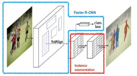
The thin layers of a deep CNN method for visual acknowledgment adopts low-level features like edges, though the deeper layers adapt more semantical ideas like faces by consolidating lower-level features. The R-CNNs perform progressive component extraction: by expanding the insight one can build the degree of reflection learned by the system. To get a thought of what is happening inside a R-CNN, Figure1 illustrates the process. It comprises of two fundamental segments: feature extraction and classification. Utilizing the mix of separating and subsampling, enlightening features are removed lastly utilized for order in the last piece of the system. The characteristics of R-CNN are listed below.
As in the R-CNN indicator, the Fast R-CNN identifier additionally utilizes a calculation like Edge Boxes to produce area recommendations. Not at all like the R-CNN indicator, which crops and resizes area recommendations, the Fast R-CNN identifier forms the whole picture. Though a R-CNN indicator must group every area, Fast R-CNN pools CNN features relating to every region proposition. Fast R-CNN is more effective than R-CNN, on the grounds that in the Fast R-CNN indicator, the calculations for covering regions are shared.
Utilize the trainFastRCNNObjectDetector capacity to prepare a Fast R-CNN object indicator. The capacity restores a fastRCNNObjectDetector that identifies objects from a picture. The Faster R-CNN indicator includes an area proposition network to produce district recommendations straightforwardly in the system instead of utilizing an outside calculation like Edge Boxes. The RPN utilizes Anchor Boxes for Object Detection. Producing region recommendations in the system is quicker and better tuned to information. The R-CNN Process is illustrated in Figure 1.
Figure 1. R-CNN process
The most settled calculation among different deep learning models is CNN, a class of neural systems that has been a prevailing strategy in PC vision assignments since the astounding outcomes were shared on the item acknowledgment known as the ImageNet Large Scale Visual Recognition Competition (ILSVRC). Obviously, there has been an overflow of interest for the capability of CNN among radiology analysts, and a few investigations have just been distributed in regions, for example, tumor discovery, characterization, division, picture recreation, and normal language processing. Recognition with this best in class system would help not just analysts who apply R-CNN to their tasks in radiology and therapeutic imaging, yet additionally clinical radiologists, as deep learning may impact their training sooner rather than existing methods. This manuscript centers around the essential ideas of R-CNN and their application to different radiology assignments, and talks about its difficulties and future enhancements.
R-CNN is a scientific development that is normally made out of three sorts of layers convolution, pooling, and completely associated layers. The initial two, convolution and pooling layers, perform feature extraction, while the third, a completely associated layer, maps the extricated features into definite result, for example, classification. A convolution layer assumes a key job in R-CNN, which is made out of a pile of numerical activities, for example, convolution, a specific kind of straight task.
R-CNN separates and extracts a lot of regions from the given picture utilizing particular search methods, and afterward checks if any of these cases contains abnormal pixels. We first concentrate these regions, and for every region, CNN is utilized to remove explicit features. At long last, these highlights are then used to recognize objects. Faster R-CNN, then again, passes the whole picture to ConvNet which produces regions of interest. Likewise, rather than utilizing three unique models, it utilizes a solitary model which concentrates features from the specified regions, orders them into various classes, and returns all bounding boxes.
All these operations are done paralley to execute quicker when contrasted with R-CNN. Fast R-CNN is, in any case, not quick enough when applied on a huge dataset as it likewise utilizes particular look for extricating the regions.
Nativ and Shaked [1] used the distinction of Gaussian channel for tumor cell recognition pursued by tough change to identify the high points. Odenaet [2] utilized chart cut based technique initialized by stones removed from Laplacian of Gaussian (LoG) channel. Radford et al. [3] proposed neighborhood isotropic stage symmetry for identification of beta cells in pancreas.
Sebag et al. [4] learn unsupervised features utilizing auto-encoders which are sustained to a classifier for cell location. Angermueller et al. [5] expanded this strategy by falling CNN and hand-made features for mitosis identification. Martinez-Torres et al. [6] proposed to restrict cores focuses utilizing a ballot system. Vondrick et al. [7] proposed a spatially compelled CNN (SCCNN) by attaching two additional layers to the completely associated layer. The additional spatially compelled layers gauge the probability of a pixel being the focal point of a core. Chen et al. [8] broadened this structure by adding hand-made features to the information which somewhat improved the F1-score and review to the loss of exactness. Van Valen et al. [9] proposed a deep relapse categorization which learns its parameters for a proximity guide produced by the division cover of mitotic cells. Roitshtain et al. [10] proposed a mix of two CNNs which perform concurrent discovery and arrangement of cells. Roitshtain et al. [11] proposed a cell thickness guide pursued by nearby maxima recognition to identify cells. As of late, Wu et al. [12] proposed a CNN which relapses an encoded feature vector that can be utilized to recoup scanty cell areas. These locations are consolidated to get the last recognition point. Litjens et al. [13] proposed an organized relapsed method to learn vicinity maps with higher qualities close to cell focuses, the nearby maxima give the focal point of cell area.
CNN give a way to deal with take in applicable features from information, as opposed to handcrafting features from the earlier. In the field of PC vision, convolutional neural systems have as of late made fast headways, showing best in class execution on an assortment of picture grouping errands. CNNs use a lot of parameterized portions to concentrate picture features, enabling particular element pieces to be scholarly for a given grouping task [14]. Thusly, CNNs can become familiar with a "portrayal" of the issue's component space. Feature space portrayals may likewise be learned in an unsupervised way via preparing CNN autoencoder engineering to encode and unravel [15]. This methodology might be valuable for learning pertinent motility features where an unequivocal arrangement errand is absent [16].
While CNNs are most generally connected to undertakings including examination of shape in two-dimensional pictures at a solitary time-point, convolution is a characteristic systematic apparatus for any info data with spatial measurements [17]. CNNs have been effectively connected to a various arrangement of non-imaging areas, including common language preparing, division, and EEG accounts. CNNs have performed well in the characterization of hand-signals from video accounts [18]. These productive executions have essentially stretched out CNNs to consider three-dimensional pictures as data sources, where one pivot is time. This methodology has additionally taken into account productive arrangement of recordings utilizing CNNs.
Tanh or Hyperbolic deviation work is a numerical limit. Park et al. [14] first used in his work. The tanh is fundamental limit and better than the sigmoid that the output is between - 1 and 1, which is to be centered around. The issue isn't causing the mixture of tendencies. It is portrayed as the relative with hyperbolic sine and cosine limits. This limit is portrayed by:
$\tanh (x)=\frac{\sinh (x)}{\cosh (x)}=\frac{e^{x}-e^{-x}}{e^{x}+e^{-x}}$ (1)
where, e is the purpose of half-yielding and half-whole of two exponential capacities [19].
Redressed direct unit is prevalent capacity. This actuation capacity has limited from zero, yet the above arrangement isn't limited disappearing inclination [20] that it is limited from zero. It will make a neuron with the inside turns out so much that you are latent neurons. It picks the limit of (0, x) characterize as:
$f(x)=\max (0, x)$ (2)
where, x is the input or training data to neuron x.
Maxout model is type of activation function and a multilayer which applying the hidden activations. Shown an input vector $x \in \Re^{d}$ and the output vector of h(x) will divide z into groups of k values [15].
$g_{i}(x)=\max _{j e[1, k]} Z_{i j}$ (3)
where, zij= xT W ij + b ij, and all are learned parameters.
Exponential Rectifier Linear Unit function is a generalization of the mean activation to zero which learn in conditions. It is better than rectified linear unit for accuracy of classification.
$h(x)=\left\{\begin{array}{l}{x} \\ {a\left(e^{x}-1\right)^{i f} x>=0 \text { otherwise }}\end{array}\right.$ (4)
where, x is a hyper-parameter to be tuned and is a >= 0 constraint.
AI designs are shaped by the piece of various direct and non-direct changes of the info information, with the objective of yielding increasingly conceptual-and at last progressively helpful portrayals [16]. These techniques have as of late turned out to be increasingly well known as they have exhibited exceptional execution in various PC vision and example acknowledgment assignments [21].
AI models are a development of multilayer neural systems, including diverse plan and preparing techniques to make them focused. These systems incorporate the consolidation of spatial invariance, various leveled feature learning and versatility [22]. A fascinating normal for this methodology is that the feature extraction is additionally considered as a piece of the learning procedure, i.e., the layers of AI models can locate an appropriate portrayal of info pictures as far as visual element maps [23, 24].
For arrangement of various kinds of movement, we apply a standard R-CNN technique using 3D convolutional and max pooling layers. 3D Convolutional layers convolve the 3D movement shape contributions with a lot of parameterized parts, passing the convolutional parameters to the layers above. The maximum pooling layers play out a maximum task for values in a 3D-window, decreasing the info size, and return the subsequent result to the layer above.
There are a few kinds of Convolutional Neural Networks (CNNs) being created and all can possibly extraordinarily add to the speed and exactness of programmed picture ID [25]. Specifically, 3D CNNs are being made to improve the distinguishing proof of moving and 3D pictures, for example, video from surveillance cameras and therapeutic sweeps of harmful tissue, a tedious procedure that as of now requires master examination [26].
Improvement of 3D CNNs is still at a beginning time because of their unpredictability, however the advantages they can convey improves the performance [27].
The feature extraction strategy is a procedure to expel completely associated layers from a system pretrained on ImageNet and keeping in mind that keeping up the rest of the system, which comprises of a progression of convolution and pooling layers, alluded to as the convolutional base, as a fixed element extractor [28].
In this situation, any AI classifier, for example, support vector machines, just as the typical completely associated layers in CNNs, can be included top of the feature extractor, bringing about preparing constrained to the additional classifier on a given dataset. This methodology isn't normal in deep learning research on medical pictures as a result of the divergence among ImageNet and given therapeutic pictures.
A tweaking strategy, which is all the more regularly connected to radiology investigation, is to not just supplant completely associated layers of the pre-trained model with another arrangement of completely associated layers [29] to retrain on a given dataset, yet to calibrate all or part of the portions in the pre-trained convolution base by methods for backpropagation [30].
Every one of the layers in the convolutional base can be adjusted or, on the other hand, some prior layers can be fixed while regulating the remainder of the deeper layers. This is roused by the perception that the early-layer features seem increasingly nonexclusive, including features, for example, edges material to an assortment of datasets and undertakings, though later features logically turned out to be progressively explicit to a specific dataset or task.
Completely associated layers are equivalent to in a customary neural system, where each perceptron unit thinks about contribution from all units in the past layer, and yields to all units in the final layer [31]. Dropout layers wipe out an irregular extent of completely associated units from a completely associated layer during each forward pass, lessening trust upon individual units and forestalling overfitting [32].
Figure 2. Tumor cells identification from images
Two completely associated layers with dropout and ReLU enactments are used at the base of the system. Last class observations are returned by a completely associated layer with various neurons equivalent to the quantity of classes and a softmax initiation. Eminently, stacking different convolutional layers is important for powerful preparing, conceivably because of the expanded open field size of more deep layers in stack. The identified tumor cells identification process from images is depicted in Figure 2.
Suppose we have discrete grayscale images and let us denote with I[x; y] the intensity of the pixel at position [x; y]. Furthermore, supposewe have Nk kernels kd of size n X n, biases bd 2 R(M||n+1) X (M||n+1) and outputs z 2R(M||n+1) X (M||n+1)/Nk. If we collect all learnable parameters in x=fλdgd=1::Nk, for λd =fkd; bdg, then the dth resulting feature map of the convolutional layer is defined as:
$\begin{aligned} g\left(m ; \theta_{d}\right):=z[m, n, d] &=\sum_{i=0}^{n-1} \sum_{j=0}^{n-1} a[m-i, n-\\j] k_{d}[i, j]+b_{d}[m, n] \end{aligned}$ (5)
Note from the size of the outputs y that this corresponds to the `valid' convolution, i.e.
$z[m, n, d]=\left(a * k_{d}\right)[m, n]+b_{d}[m, n]$ (6)
To mean the real contribution with I0 and the result after the kth layer with Ik. We need to investigate what the successful responsive field is on I0, in the event that we apply a convolution on I1. In the event that we apply a 3 X 3 convolution on I1, the portions will cover the entire picture in one stage.
Since use of convolutional layers with pieces of estimate 3 X 3, these layers scale back a N X N measured contribution to (N α 3+1) X (N α 3+1). In the event that we acquire a 3 X 3 measured picture as I1, at that point we can without much of a stretch tackle Nα3+1=3 to get N=5.
While applying 2D convolutions like 3X3 convolutions on images, a 3X3 convolution filter, in general will always have a third dimension in size. This filter depends on the number of channels of the input image. So, we apply a 3X3X1 convolution filter on gray-scale images whereas, we apply a 3X3X3 convolution filter on a colored image.
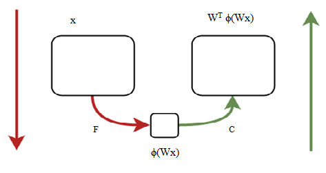
Now Auto-encoders are prepared with back-proliferation to remake their contribution from an inert variable portrayal. So albeit no ground-truth is accessible AEs structure their own objectives as y(i)=x(i).
Rather than basically learning the character mapping, an auto-encoder is compelled to initially encode the information in a compacted portrayal, and therefore interpret from this packed portrayal. Due to this pressure, it must make a determination of the most significant features for reproduction, and will subsequently learn structure about the information.
Auto-encoders are characterized as a neural system with encoder F: Rn ! Rh, parametrized by F, and decoder C: Rh ! Rn, parametrized by C. The forward pass is again given by
f(x)=C(F(x)) (7)
Regularly we have either h < n, or h > n and F is compelled to get familiar with a meager portrayal in Rh. Auto-encoders generally limit the squared reproduction error with a regularization which is represented as:
$\min _{\theta=\left\{\theta_{F}, \theta_{C}\right\}} \frac{1}{N} \sum_{i=1}^{N}\left|C\left(F\left(x^{(i)} ; \theta_{F}\right) ; \theta_{C}\right)-x^{(i)}\right|_{2}^{2}+\lambda J(\theta)$ (8)
Numerous kinds of auto-encoders have been proposed throughout the years, of which the least difficult one is a conventional neural system with only one shrouded layer thus called tied-loads, for a perception. Taking tied-loads implies that we take the transpose of the weight grid from the encoder as weight network for the decoder.
The proposed model extracts the features x from the image data set ϕ(Wx) and form a set x of features f from the cluster C. The process is depicted below in Figure 3 and feature subset formation is depicted in Figure 4.
Figure 3. Feature extraction process
Figure 4. Feature subset Formation
Auto-encoders join information with separating parameters with similar values. Sifting coefficients in these premise portrayals adds up to intensifying or lessening explicit properties or examples of the info signal, while sparsifying the portrayal that adds up to a type of measurement.
A large portion of the discrete variants of these techniques can be composed as a symmetrical projection into an outrageous area, trailed by a separating in the repugnant space, lastly pursued by a projection once more into the information area. For instance, let us think about the sifting of a sign x by methods for a convolution with a piece k. The CNN architecture for tumor cell classification is depicted in Figure 5.
Figure 5. CNN architecture for tumor cell classification
3.1 Machine learning based Algorithm for Tumor cell identification
The proposed algorithm for tumor cell identification is illustrated below.
Input: F(I1,I2,……Im),T $\theta$ // Relevant Threshold
Output: FS //feature subset
Begin:
For i=1 to m do
For j=i to n do
Relevantf= ML(Ii,T,maxcount)
{
FS= fset(ΔTree, F )
}
end for
end for
If Relevantf>$\theta$
Append fi to FS
end if
G’=Arrange ML (I, T, maxcount) in ascending order.
FS=fset (ΔTree, Y, L, G’)
fset (ΔTree, Y, L, G’)
{
F=ΔTree.Ti Node;
For every feature Ii$\in$ FS
Extract ML (Fi; Fn)
end for
}
end fset;
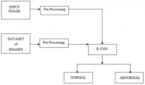
Initially an image dataset is given as input and the feature set FS will be generated as output which identifies the tumor cells. Based on R-CNN method the threshold images given construct a tree (ΔTree) and stored in the system. The below figure represents the process.
The tree construction using R-CNN is clearly depicted in Figure 6. After constructing the tree, the machine is capable of recognizing the tumor cells, then a dataset with images are given as input and then from the images, features are extracted and a feature subset is generated. In the proposed algorithm, I is the image and T is the threshold value and max count represent the number of images in the dataset. Y is the image considered and L is the image represented as tree and G is the parameters considered. Based on the images provided, the R-CNN method generates a FS (feature subset).
Figure 6. Tree construction using R-CNN
To decide whether CNNs can recognize more contrasts in cell state, classifiers were prepared to separate among MuSCs and myoblasts (n=225 for every class) to decide whether CNNs could be utilized to distinguish various conditions of myogenic duty. Movement shapes were evenly and vertically turned to expand preparing set assorted variety without irritating the portrayal of motility. The proposed method is implemented in python using ANACONDA SPYDER Platform. The results show that the proposed method is better than the existing methods.
Results so far show that managed grouping of various cell motility phenotypes utilizing convolutional neural systems is viable, and that standard unique information increase and learning methods perform well. In any case, in the investigation of motility information, regulated grouping information isn't constantly accessible.
For example, to investigate the heterogeneity of phenotypes in a given populace, there is no conspicuous strategy to produce managed arrangement information that might be utilized to learn applicable component portions [33] by enhancement of a standard grouping. This would likewise be an issue in the ID of heterogeneous motility practices in patient biopsy tests, in which the distinctive features are not known from the earlier. The parameters used in the dataset are depicted in Table 1.
In order to assess the efficiency of our proposed method various evaluation metrics are utilized. The metrics consists of group of esteems that contains normal primary evaluating methods [34, 35]. The evaluation metrics used here contains True Positive, True Negative, False Positive and False Negative, Sensitivity, Specificity and Accuracy [36].
The proposed method detects the tumor cells and separates them from the normal cells. The cells are formed as a separate cluster for both tumor and non-tumor cells. The clusters are depicted in Figure 7.
Using R-CNN with autoencoders in an unsupervised manner has been utilized in different settings to learn important features where no conspicuous grouping issue is available. We next endeavored to prepare autoencoders on our 3D portrayals of tumor cell motility to learn applicable component bits without a directed grouping issue.
Table 1. Parameters in dataset
|
Variable |
Total population |
ETV4 |
P-value |
|
|
Under expression |
Over expression |
|||
|
Total Median age(range), years Age,n(%) $\leq$ 35 years >35 years Menopausal status,n(%) Premenopausal Premenopausal Tumor size,n(%) $\leq$ 2cm >2cm Lymph nodes status,n(%) Negative Positive AJCC stage,n(%) VII III Histological grade,n(%) VII III Lympho vascular invasion,n(%) Yes No |
135 49(16-76)
31(23.0) 104(77.0)
78(57.8) 57(42.2)
33(24.4) 102(75.6)
63(46.7) 72(53.3)
93(68.9) 42(31.1)
39(28.9) 96(71.1)
36(26.7) 99(73.3)
|
58(43.0) 49(27-76)
15(48.4) 43(41.3)
34(43.6) 24(42.1)
18(54.5) 40(39.2)
37(58.7) 21(29.2)
52(55.9) 6(14.3)
20(51.3) 38(39.6)
8(22.2) 50(50.5) |
77(57.0) 49(16-72)
16(51.6) 61(58.7)
44(56.4) 33(57.9)
15(45.5) 62(60.8)
26(41.3) 51(70.8)
41(44.1) 36(85.7)
19(48.7) 58(60.4)
28(77.8) 49(49.5)2 |
0.641 (Mann-Whitney)
0.311
0.502
0.090
<0.0001
<0.0001
0.146
0.003 |
Table 2. Tumor identification parameters ranges
|
Features Selected |
Performance measure Using SVM |
Performance measure for SVM with Polynomial |
Performance measure for ANN |
Performance measure Using R-CNN with auto encoders |
||||||||
|
Accuracy |
Sensitivity |
Specificity |
Accuracy |
Sensitivity |
Specificity |
Accuracy |
Sensitivity |
Specificity |
Accuracy |
Sensitivity |
Specificity |
|
|
50 |
99.18% |
100.00% |
98.71% |
98.78% |
98.99% |
98.71% |
97.44% |
96.43% |
100.00% |
98.68% |
100.00% |
97.78% |
|
100 |
98.80% |
100.00% |
98.04% |
100.00% |
100.00% |
100.00% |
97.44% |
96.15% |
100.00% |
97.37% |
96.77% |
97.78% |
|
All |
98.75% |
100.00% |
98.00% |
99.18% |
99.00% |
99.33% |
92.05% |
90.91% |
100.00% |
98.68% |
100.00% |
97.78% |
Figure 7. Tumor and non-tumor cells cluster
$\begin{array}{c}{\text { Sensitivity }=\frac{\mathrm{T}(\mathrm{P})}{\mathrm{T}(\mathrm{P})+\mathrm{F}(\mathrm{N})}} \\ {\text { Specificity }=\frac{\mathrm{T}(\mathrm{N})}{\mathrm{F}(\mathrm{P})+\mathrm{T}(\mathrm{N})}} \\ {\text { Accuracy }=\frac{\mathrm{T}(\mathrm{P})+\mathrm{T}(\mathrm{N})}{\mathrm{T}(\mathrm{P})+\mathrm{F}(\mathrm{N})+\mathrm{F}(\mathrm{P})+\mathrm{T}(\mathrm{N})}}\end{array}$
A standard autoencoder using stacked convolutions, trailed by upsampling and stacked convolutional layers was prepared on 13,500 examples of each class for three sorts of recreated movement. The Table 2 depicts the values of different parameters for tumor cell identification.
The Figure 8 illustrates the comparison levels of different classifiers. The picture below show that the proposed method performance is better than the existing methods.
To decide whether autoencoders prepared on 3D motility portrayals could be utilized as feature extractors, we used the result of the autoencoder's focal layer as features. Features from the focal point of this autoencoder seem valuable for class division when the element space is envisioned.
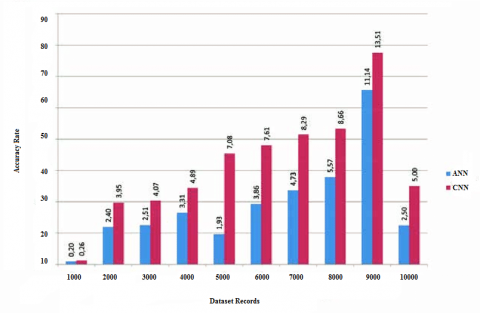
The accuracy rate of the proposed and traditional methods is depicted in Figure 9. The accuracy rate of the proposed method is high when compared with the existing methods. The results show that the proposed method is far better than the traditional methods.
Convolutional neural networks take into account learning, or learning of features applicable for the depiction of a component space in tumor cells. We show that R-CNNs are fit for separating between reenacted models of movement and different sorts of cell motility. Also, we find that R-CNN autoencoders can be prepared adequately on these 3D movement portrayals in an unsupervised manner. In our cell informational indexes, we find that CNNs adequately segregate between various cell types, and various conditions of myogenic predecessor actuation. While we apply the techniques portrayed here to cell science, there is no theoretical confinement that avoids application to different fields where segregation dependent on movement accounts. Despite the fact that there are a few strategies that encourage learning on littler datasets as depicted above, well-commented on enormous medicinal datasets are as yet required since a large portion of the eminent achievements of deep learning are normally founded on a lot of information. The proposed R-CNN method using auto encoders performs better when compared to traditional data mining and Artificial Intelligence (AI) methods.
[1] Nativ, A., Shaked, N.T. (2017). Compact interferometric module for full-field interferometric phase microscopy with low spatial coherence illumination. Optics Letters, 42(8): 1492-1495. https://doi.org/10.1364/OL.42.001492
[2] Odena, A. (2016). Semi-supervised learning with generative adversarial networks. arXiv preprint arXiv:1606.01583.
[3] Radford, A., Metz, L., Chintala, S. (2015). Unsupervised representation learning with deep convolutional generative adversarial networks. arXiv preprint arXiv:1511.06434.
[4] Sebag, A.S., Plancade, S., Raulet-Tomkiewicz, C., Barouki, R., Vert, J.P., Walter, T. (2015). A generic methodological framework for studying single cell motility in high-throughput time-lapse data. Bioinformatics, 31(12): 320-328. https://doi.org/10.1093/bioinformatics/btv225
[5] Angermueller, C., Parnamaa, T., Parts, L., Stegle, O. (2016). Deep learning for computational biology. Molecular Systems Biology, 12(7): 878. https://doi.org/10.15252/msb.20156651
[6] Martinez-Torres, C.E., Laperrousaz, B., Berguiga, L., Boyer-Provera, E., Elezgaray, J., Nicolini, F.E., Maguer-Satta, V., Arneodo, A., Argoul, F. (2015). Deciphering the internal complexity of living cells with quantitative phase microscopy: A multiscale approach. Journal of Biomedical Optics, 20(9): 096005. https://doi.org/10.1117/1.JBO.20.9.096005
[7] Vondrick, C., Pirsiavash, H., Torralba, A. (2016). Generating videos with scene dynamics. Advances in Neural Information Processing Systems, 613-621.
[8] Chen, C.L., Mahjoubfar, A., Tai, L.C., Blaby, I.K., Huang, A., Niazi, K.R., Jalali, B. (2016). Deep learning in label-free cell classification. Scientific Reports, 6: 21471. https://doi.org/10.1038/srep21471
[9] Van Valen, D.A., Kudo, T., Lane, K.M., Macklin, D.N., Quach, N.T., DeFelice, M.M., Maayan, I., Tanouchi, Y., Ashley, E.A., Covert, M.W. (2016). Deep Learning Automates the Quantitative Analysis of Individual Cells in Live-Cell Imaging Experiments. PLoS Computational Biology, 12(11): e1005177. https://doi.org/10.1371/journal.pcbi.1005177
[10] Roitshtain, D., Wolbromsky, L., Bal, E., Greenspan, H., Satterwhite, L.L., Shaked, N.T. (2017). Quantitative phase microscopy spatial signatures of cancer cells. Cytometry Part A, 91(5): 482-493. https://doi.org/10.1002/cyto.a.23100
[11] Roitshtain, D., Turko, N.A., Javidi, B., Shaked, N.T. (2016). Flipping interferometry and its application for quantitative phase microscopy in a micro-channel. Optics Letters, 41(10): 2354-2357. https://doi.org/10.1364/OL.41.002354
[12] Wu, D., Pigou, L., Kindermans, P.J., Le, N.D., Shao, L., Dambre, J., Odobez, J.M. (2016). Deep dynamic neural networks for multimodal gesture segmentation and recognition. IEEE Transactions on Pattern Analysis and Machine Intelligence, 38(8): 1583-1597. https://doi.org/10.1109/TPAMI.2016.2537340
[13] Litjens, G., Kooi, T., Bejnordi, B.E., Setio, A.A.A., Ciompi, F., Ghafoorian, M., van der Laak, J.A.W.M., van Ginneken, B., Sanchez, C.I. (2017). A survey on deep learning in medical image analysis. Medical Image Analysis, 42: 60-88. https://doi.org/10.1016/j.media.2017.07.005
[14] Park, S., Rinehart, M.T., Walzer, K.A., Chi, J.T.A., Wax, A. (2016). Automated detection of P. falciparum using machine learning algorithms with quantitative phase images of unstained cells. PLoS ONE, 11(9): e0163045. https://doi.org/10.1371/journal.pone.0163045
[15] Shin, H.C., Roth, H.R., Gao, M., Lu, L., Xu, Z., Nogues, I., Yao, J., Mollura, D., Summers, R.M. (2016). Deep convolutional neural networks for computer-aided detection: CNN architectures, dataset characteristics and transfer learning. IEEE Tran Med Imaging, 35(5): 1285-1298. https://doi.org/10.1109/TMI.2016.2528162
[16] Howard, A.G., Zhu, M., Chen, B., Kalenichenko, D., Wang, W., Weyand, T., Andreetto, M., Adam, H. (2017). MobileNets: Efficient convolutional neural networks for mobile vision applications. arXiv preprint, arXiv:1704.04861.
[17] Shi, J., Zhou, S., Liu, X., Zhang, Q., Lu, M., Wang, T. (2016). Stacked deep polynomial network based representation learning for tumor classification with small ultrasound image dataset. Neurocomputing, 194: 87-94. https://doi.org/10.1016/j.neucom.2016.01.074
[18] Yoon, J., Jo, Y.J., Kim, M., Kim, K., Lee, S.Y., Kang, S.J., Park, Y.K. (2017). Identification of non-activated lymphocytes using three-dimensional refractive index tomography and machine learning. Scientific Reports, 7(1): 6654. https://doi.org/10.1038/s41598-017-06311-y
[19] Yosinski, J., Clune, J., Bengio, Y. (2014). How transferable are features in deep neural networks?. Advances in Neural Information Processing Systems.
[20] Ng, J.Y.H., Hausknecht, M., Vijayanarasimhan, S., Vinyals, O., Monga, R., Toderici, G. (2015). Beyond short snippets: Deep networks for video classification. 2015 IEEE Conference on Computer Vision and Pattern Recognition (CVPR), pp. 4694-4702. https://doi.org/10.1109/CVPR.2015.7299101
[21] He, K., Zhang, X., Ren, S., Sun, J. (2016). Deep residual learning for image recognition. The IEEE Computer Society Conference on Computer Vision and Pattern Recognition, pp. 770-778.
[22] Frid-Adar, M., Diamant, I., Klang, E., Amitai, M., Goldberger, J., Greenspan, H. (2018). GAN-based synthetic medical image augmentation for increased CNN performance in liver lesion classification. Neurocomputing, 321: 321-331. https://doi.org/10.1016/j.neucom.2018.09.013
[23] Hejna, M., Jorapur, A., Song, J.S., Judson, R.L. (2017). High accuracy label-free classification of single-cell kinetic states from holographic cytometry of human melanoma cells. Scientific Reports, 7(1): 11943. https://doi.org/10.1038/s41598-017-12165-1
[24] Tierney, M.T., Sacco, A. (2016). Satellite Cell Heterogeneity in Skeletal Muscle Homeostasis. Trends in Cell Biology, 26(6): 434-444. https://doi.org/10.1016/j.tcb.2016.02.004
[25] Bray, M.A., Carpenter, A.E. (2015). CellProfiler Tracer: exploring and validating high-throughput, time-lapse microscopy image data. BMC Bioinformatics, 16(1): 368. https://doi.org/10.1186/s12859-015-0759-x
[26] Tajbakhsh, N., Shin, J.Y., Gurudu, S.R., Hurst, R.T., Kendall, C.B., Gotway, M.B., Liang, J. (2016). Convolutional neural networks for medical image analysis: Full training or fine tuning. IEEE Transactions on Medical Imaging, 35(5): 1299-1312. https://doi.org/10.1109/TMI.2016.2535302
[27] Ronneberger, O., Fischer, P., Brox, T. (2015). U-net: Convolutional networks for biomedical image segmentation. International Conference on Medical Image Computing and Computer-Assisted Intervention: 234-241. https://doi.org/10.1007/978-3-319-24574-4_28
[28] Wu, P.H., Phillip, J.M., Khatau, S.B., Chen, W.C., Stirman, J., Rosseel, S., Tschudi, K., Van Patten, J., Wong, M. Gupta, S. (2015). Evolution of cellular morpho-phenotypes in cancer metastasis. Scientific Reports, 5: 18437. https://doi.org/10.1038/srep18437
[29] Mirsky, S.K., Barnea, I., Levi, M., Greenspan, H., Shaked, N.T. (2017). Automated analysis of individual sperm cells using stain-free interferometric phase microscopy and machine learning. Cytometry Part A, 91(9): 893-900. https://doi.org/10.1002/cyto.a.23189
[30] Go, T., Kim, J.H., Byeon, H., Lee, S.J. (2018). Machine learning-based in-line holographic sensing of unstained malaria-infected red blood cells. Biophotonics, 11(9): e201800101. https://doi.org/10.1002/jbio.201800101
[31] Salimans, T., Goodfellow, I., Zaremba, W., Cheung, V., Radford, A., Chen, X. (2016). Improved techniques for training gans. Advances in Neural Information Processing Systems.
[32] Ahsan, U., Sun, C., Essa, I. (2018). Discrimnet: Semi-supervised action recognition from videos using generative adversarial networks. arXiv preprint, arXiv: 1801.07230.
[33] Lam, V.K., Nguyen, T.C., Chung, B.M., Nehmetallah, G., Raub, C.B. (2017). Quantitative assessment of cancer cell morphology and motility using telecentric digital holographic microscopy and machine learning. Cytometry Part A, 93(3): 334-345. https://doi.org/10.1002/cyto.a.23316
[34] Jo, Y.J., Cho, H., Lee, S.Y., Choi, G., Kim, G., Min, H., Park, Y. (2019). Quantitative phase imaging and artificial intelligence: A review. IEEE Journal of Selected Topics in Quantum Electronics, 25(1): 1-14. https://doi.org/10.1109/JSTQE.2018.2859234
[35] Rivenson, Y., Liu, T., Wei, Z., Zhang, Y., Ozcan, A. (2019). PhaseStain: Digital staining of label-free quantitative phase microscopy images using deep learning. Light: Science & Applications, 23. https://doi.org/10.1038/s41377-019-0129-y
[36] Rivenson, Y., Zhang, Y., Gunaydin, H., Teng, D., Ozcan, A. (2018). Phase recovery and holographic image reconstruction using deep learning in neural networks. Light: Science & Applications, 7. https://doi.org/10.1038/lsa.2017.141