Laid Chergui* | Saad Bouguezel
© 2019 IIETA. This article is published by IIETA and is licensed under the CC BY 4.0 license (http://creativecommons.org/licenses/by/4.0/).
OPEN ACCESS
This paper proposes a new post-whitening transform domain LMS (POW-TDLMS) algorithm for system identification purposes, where the post whitened and original transformed signals are used during the adaptation and filtering phases, respectively. The main idea behind the proposed algorithm is to introduce a first order adaptive post-whitening filter in the TDLMS algorithm after applying the transform to completely decorrelate the transformed signal. Linear prediction is adopted for the post-whitening and the prediction coefficients are adapted in the time domain. Furthermore, the mean convergence performance analysis of the proposed POW-TDLMS algorithm is presented. The simulation results show the superiority of the proposed POW-TDLMS algorithm compared to the conventional TDLMS algorithm in terms of the MSE convergence speed and reached steady state.
eigen-value spread, orthogonal transforms, post-whitening, predictive decorrelation, system identification, TDLMS
The least mean square (LMS) algorithm is an adaptive filtering algorithm known for its simplicity, robustness and low computational complexity [1-3]. The convergence of this algorithm becomes slow in the case of correlated input signals. The autocorrelation matrix of such signals is said ill conditioned [4-6].
In the literature, several solutions and alternatives have been proposed to improve the performance of the LMS algorithm when it is employed with correlated input signals. In [7], Mboub et al. proposed a new whitening structure for the acoustic echo cancellation. In [8, 9], the authors devised a pre-whitening for the time domain LMS algorithm and its variants. The resulting pre-whitening techniques have allowed improvements in the convergence performance. The affine projection algorithms were developed to speed up the convergence of the gradient based algorithms in the case of correlated input signals [1, 10].
In [11], Narayan et al. proposed a new LMS algorithm operating in the transform domain, where orthogonal and unitary transforms have been used for the decorrelation of the input signal. The transformed signal is then normalised by its power, which allows the reduction of the eigenvalue spread of the autocorrelation matrix of the resulting signal, and thus offers improvements in the convergence performance of the resulting algorithm called transform domain LMS algorithm (TDLMS) [12]. The convergence performance of the TDLMS algorithm depends on the used orthogonal transforms, which are known to be limited in terms of decorrelation [13, 14]. In [13], Chergui et Bouguezel proposed a new pre-whitening (PW) of the TDLMS (PW-
TDLMS) algorithm. This pre-whitening allows the reinforcement of the decorrelation of the used orthogonal transforms, and consequently the improvements in the convergence performance of the corresponding PW-TDLMS algorithms. The PW-TDLMS algorithm was intended for applications of adaptive noise cancellation in the speech signal, where the pre-whitened and transformed signal is used during both filtering and adaptation phases. However, the PW-TDLMS algorithm cannot be applied in system identification applications, where the input signal characteristics must not be changed before the filtering phase [15, 16] and may only be modified during the adaptation phase.
In this paper, to deal with system identification applications, we propose a post-whitening (POW) of the TDLMS algorithm to ensure further decorrelation of the transformed signal and significantly reinforce the decorrelation of the used orthogonal transforms. The post-whitening process is designed using a first order adaptive decorrelation filter based on linear prediction and the prediction coefficients are adapted in the time domain. In the proposed algorithm, the post whitened and original transformed signals are used during the adaptation and filtering phases, respectively. This allows improvements in the convergence performance of the TDLMS algorithm in system identification applications.
This paper is organized as follows: Section 2 gives a review of the conventional TDLMS algorithm. Section 3 proposes a new post-whitening TDLMS (POW-TDLMS) algorithm. Section 4 presents a study of the mean convergence performance of the proposed POW-TDLMS algorithm. Section 5 discusses the simulation results. Finally, the conclusion is given in Section 6.
The conventional TDLMS algorithm presented in Figure 1 can be summarised as [17, 18]:
Let $\mathbf{x}_{k}^{N}=\left[x_{k}, x_{k-1}, \ldots, x_{k-N+1}\right]^{T}$ be the input signal of length N, where $( .)^{T}$ denotes the transposition operation. Its transformed version $\mathbf{X}_{k}^{N}$ is also of length N and obtained using the $N \times N$ orthogonal transform matrix $\mathbf{T}_{N}$ as
$\mathbf{X}_{k}^{N}=\mathbf{T}_{N} \mathbf{x}_{k}^{N}=\left[\mathbf{X}_{k}(0), \mathbf{X}_{k}(1), \ldots, \mathbf{X}_{k}(N-1)\right]^{T}$ (1)
Figure 1. Block diagram of the TDLMS adaptive filter [13, 18]
The sample $y_{k}$ at the output of the filter is obtained as
$y_{k}=\left(\mathbf{w}_{k}^{N}\right)^{H} \mathbf{X}_{k}^{N}$ (2)
where, $( .)^{H}$ denotes the complexe conjugate transpose operation and $\mathbf{w}_{k}^{N}=\left[w_{k}(0), w_{k}(1), \ldots, w_{k}(N-1)\right]^{T}$ is the filter vector of length $N$ , which is updated at each instant sample $k$ according to the adaptation equation given by
$\mathbf{w}_{k+1}^{N}=\mathbf{w}_{k}^{N}+\mu e_{k} \mathbf{P}_{k}^{-1} \mathbf{X}_{k}^{N}$ (3)
with $e_{k}=d_{k}-y_{k}$ being the sample of the error signal and $d_{k}$ is the sample of the desired signal, $\mathbf{P}_{k}=\operatorname{diag}\left(\sigma_{k}^{2}(0), \sigma_{k}^{2}(1), \ldots, \sigma_{k}^{2}(N-1)\right)$, the entries $\sigma_{k}^{2}(i)$, $i=0,1, \ldots, N-1,$ are obtained from the power estimate $\boldsymbol{\sigma}_{k}^{2}=\left[\sigma_{k}^{2}(0), \sigma_{k}^{2}(1), \ldots, \sigma_{k}^{2}(N-1)\right]^{T}$ of $\mathbf{X}_{k}^{N}$, which can be computed recursively at each time sample $k$ as $\sigma_{k}^{2}(i)=\beta \sigma_{k-1}^{2}(i)+(1-\beta)\left|\mathrm{X}_{k}(i)\right|^{2}, \beta$ is a smoothing factor that takes values in the interval $] 0,1[$. The matrix $\mathbf{P}_{k}$ is used for normalising the transformed signal and the constant step size $\mathcal{L}$ is employed for controlling the MSE convergence of the TDLMS algorithm.
2.1 Convergence analysis
In this subsection we briefly review the convergence analysis with first order autoregressive (AR1) process. The signal $\mathbf{x}_{k}$ obtained from the AR1 process is defined at each instant sample k as [13, 20, 21]:
$x_{k}=\rho x_{k-1}+\omega_{k}$ (4)
where, $\rho$ is the correlation coefficient that takes values in the interval $\left[01\left[\text { and } \omega_{k}\right.\right.$ is a stationary white Gaussian noise with variance that makes the power of $\mathbf{x}_{k}$ equal to 1.
The autocorrelation matrix of the input signal $\mathbf{x}_{k}$ is defined as:
$\mathbf{R}_{N}=\left(\begin{array}{ccccc}{1} & {\rho} & {\rho^{2}} & {\dots} & {\rho^{N-1}} \\ {\rho} & {1} & {\rho} & {\cdots} & {\rho^{N-2}} \\ {\rho^{2}} & {\rho} & {1} & {} & {} \\ {\vdots} & {\vdots} & {} & {\ddots} & {\vdots} \\ {\rho^{N-1}} & {\rho^{N-2}} & {} & {\cdots} & {1}\end{array}\right)$ (5)
The eigenvalue spread of $\mathbf{R}_{N}$ is defined as:
$\lim _{N \rightarrow \infty}\left(\text { Eigenvalue spread of } \mathbf{R}_{N}\right)=\left(\frac{1+\rho}{1-\rho}\right)^{2}$ (6)
A high value of $\rho$ inceases the correlation of $\mathbf{x}_{k},$ and consequently increases the eigenvalue spread of the autocorrelation matrix $\mathbf{R}_{N}$ . The orthogonal transforms namely the DCT, the DFT and the DHT are used in the TDLMS as a decorrelator, which allows the whitening of the input signal $\mathbf{x}_{k}$ , before being used by the LMS algorithm and consequently improves the convergence performances of the TDLMS algorithm. The autocorrelation matrix of the transformed signal and normalised by its power is defined as:
$\mathbf{S}_{N}=\left(\operatorname{diag}\left(\mathbf{B}_{N}\right)\right)^{-\frac{1}{2}} \mathbf{B}_{N}\left(\operatorname{diag}\left(\mathbf{B}_{N}\right)\right)^{-\frac{1}{2}}$ (7)
and $\mathbf{B}_{N}=\mathbf{T}_{N} \mathbf{R}_{N} \mathbf{T}_{N}^{H}$.
The eigenvalue spreads of "S" _"N" are defined for various transforms as:
$\lim _{\mathrm{N} \rightarrow \infty}\left(\begin{array}{c}{\text { Eigenvalue spread after DFT or }} \\ {\text { DHT and power normalisation }}\end{array}\right)=\left(\frac{1+\rho}{1-\rho}\right)$ (8)
$\lim _{\mathrm{N} \rightarrow \infty}\left(\begin{array}{c}{\text { Eigenvalue spread after DFT or }} \\ {\text { DHT and power normalisation }}\end{array}\right)=\left(\frac{1+\rho}{1-\rho}\right)$ (9)
The different transforms significantly decrease the eigenvalue spread of the autocorrelation matrix $\mathbf{S}_{N}$ and the DCT is considered as suboptimal in terms of decorrelation and offers the best reduction in the eigenvalue spread of $\mathbf{S}_{N}$ compared to the DFT and the DHT transforms.
3.1 Proposed post-whitening approach
The decorrelation based on the linear prediction is given in time domain as [9, 13]
$\tilde{x}_{k}=x_{k}-\left(\begin{array}{c}{L-1} \\ {k-1}\end{array}\right)^{T} \mathbf{x}_{k-1}^{L-1}$ (10)
where, $x_{k-1}^{L-1}=\left[x_{k+1}, x_{k 2}, \ldots, x_{k k+1}\right]^{T}$ is the input sub-sequence of length $L-1,$ which is supposed to be correlated, and $a_{k-1}^{L-1}=\left[a_{k-1}(1), a_{k-1}(2), \ldots, a_{k-1}(L-1)\right]^{T}$, which can be computed adaptively at each time sample $k$ using LMS algorithm as
$a_{k}^{L-1}=a_{k-1}^{L-1}+\gamma \tilde{x}_{k} x_{k-1}^{I-1}$ (11)
with $\gamma$ being the adaptation step size parameter. The decorrelation filter used in Eq $(10)$ is of order $L-1$ and has a finite impulse response (FIR) $\left[1,-\left(a_{k-1}^{L-1}\right)^{T}\right]$ of length $L$ Using Eq $(10),$ the preceding $N-1$ samples of $\tilde{x}_{k}$ can be obtained by decorrelating the preceding $N-1$ samples of $x_{k}$ as $\nu$
$\tilde{x}_{k-1}=x_{k-1}-\left(a_{k-2}^{L-1}\right)^{T} \mathbf{x}_{k-2}^{L-1}$
$\vdots$$\vdots$
$\tilde{x}_{k-N+1}=x_{k-N+1}-\left(a_{k-N}^{L-1}\right)^{T} \mathbf{x}_{k-N}^{L-1}$ (12)
Therefore, Eq. (10) and Eq. (12) can be combined and compactly formulated as
$\tilde{\mathbf{x}}_{k}^{V}=\mathbf{x}_{k}^{N}-\left[\left(a_{k-1}^{L-1}\right)^{T} \mathbf{x}_{k-1}^{L-1},\left(a_{k-2}^{L-1}\right)^{T} \mathbf{x}_{k-1}^{L-1} \ldots\left(a_{k k}^{L-1}\right)^{T} \mathbf{x}_{k-1}^{L-1}\right]^{T}$ (13)
It is clear that the decorrelation in Eq. (13) is achieved using the FIR decorrelation filters $\left[1,-\left(a_{k-1}^{L-1}\right)^{T}\right]_{,[1,2] m}\left[1,-\left(a_{k-2}^{L-1}\right)^{T}\right], \ldots,$ and $\left[1,-\left(a_{k-1}^{L-1}\right)^{T}\right]$ of order $L-1$ . Finally, by multiplying both sides $\text { of order } L-1 . \text { Finally, by multiplying both sides of Eq ( } 13)$ by $\mathrm{T}_{N}$ , the proposed post-whitening of the transformed signal $\mathrm{X}_{k}^{N}$ can be obtained as
$\widetilde{\mathbf{X}}_{k}^{N}=\mathbf{X}_{k}^{N}-\mathbf{T}_{N} \times\left[\left(\boldsymbol{a}_{k-1}^{L-1}\right)^{T} \mathbf{x}_{k-1}^{L-1},\left(\boldsymbol{a}_{k-2}^{L-1}\right)^{T} \mathbf{x}_{k-2}^{L-1}, \ldots,\left(\boldsymbol{a}_{k-N}^{L-1}\right)^{T} \mathbf{x}_{k-N}^{L-1}\right]^{T}$ (14)
For simplicity, we consider in this paper the case of first order decorrelation filters, i.e. $L=2$ . Thus, Eq. (14) becomes
$\widetilde{\mathbf{X}}_{k}^{N}=\mathbf{X}_{k}^{N}-\mathbf{T}_{N} \times\left[a_{k-1}(1) x_{k-1}, a_{k-2}(1) x_{k-2} \ldots, a_{k-1}(1) x_{k-N}\right]^{T}$
$=\mathbf{X}_{k}^{N}-\mathbf{T}_{N} \times \operatorname{diag}\left(a_{k-1}(1), a_{k-2}(1), \ldots, a_{k-N}(1)\right) \mathbf{x} \mathbf{x}_{k-1}^{N}$ (15)
Figure 2. Proposed first order adaptive post-whitening
In this case $(L=2),$ the prediction coefficients $a_{k-i}(1), i=1,2, \ldots, N$, in Eq. (15) are computed using the simplified versions of Eq. (10) and Eq. (11) as
$\tilde{x}_{k}=x_{k}-a_{k-1}(1) x_{k-1}$ (16)
$a_{k}(1)=a_{k-1}(1)+\gamma \tilde{x}_{k} x_{k-1}$ (17)
Therefore, Eq. (15), Eq. (16) and Eq. (17) represent the first order adaptive post–whitening process of the transformed signal $\mathbf{X}_{k}^{N}$ , which is illustrated by Figure 2, where the input signal $\mathbf{x}_{k-1}^{N}=\left[x_{k-1}, x_{k-2}, \ldots, x_{k-N}\right]^{T}$ is weighted using the prediction coefficients $a_{k-i}(1), i=1,2, \ldots, N$, before being transformed by $\mathbf{T}_{N}$ and the resulting vector is subtracted from $\mathbf{X}_{k}^{N}$ to provide the post-whitened signal $\widetilde{\mathbf{X}}_{k}^{V}=\left[\widetilde{\mathrm{X}}_{k}(0), \widetilde{\mathrm{X}}_{k}(1), \ldots, \widetilde{\mathrm{X}}_{k}(N-1)\right]^{T}$ .
3.2 Proposed post whitening TDLMS algorithm
In this subsection, we introduce the proposed post-whitening given by Eq. (15), Eq. (16), Eq. (17) and Figure 2 in the TDLMS to develop a new Post-whitening TDLMS (POW-TDLMS) algorithm to reinforce the decorrelation of the used orthogonal transform $\mathbf{T}_{N}$ , and consequently, to decrease the eigenvalue spread of the autocorrelation matrix of the post whitened signal $\tilde{\mathbf{X}}_{k}^{N}$ normalised by its power. Therefore, the convergence performance of the TDLMS would be improved in terms of the MSE convergence behaviour.
Figure 3. Proposed post-whitening TDLMS algorithm
After introducing the proposed post-whitening approach, we develop the proposed POW-TDLMS algorithm for system identification as shown in Figure 3, where $v_{k}$ is the observation noise generated from a random white Gaussian process, and $\mathbf{h}=[h(0), h(1), \ldots, h(N-1)]^{T}$ is the unknown system impulse response to be identified by the adaptive filter.
In Figure 3, the error signal at the output of the filter is given by
$e_{k}=d_{k}-\left(\mathbf{w}_{k}^{N}\right)^{H} \mathbf{X}_{k}^{N}$ (18)
and the desired signal is given by
$d_{k}=v_{k}+\sum_{i=0}^{N-1} h(i) x_{k-i}$ (19)
The post-whitened signal $\widetilde{\mathbf{X}}_{k}^{N}$ is normalised by its power defined as
$\widetilde{\mathbf{P}}_{k}=\operatorname{diag}\left(\left[\tilde{\sigma}_{k}^{2}(0), \tilde{\sigma}_{k}^{2}(1), \ldots, \tilde{\sigma}_{k}^{2}(N-1)\right]\right)$ (20)
where,$\tilde{\sigma}_{k}^{2}(i)$ is the estimation of the power of the $i^{\mathrm{th}}$ input $\overline{\mathrm{X}}_{k}(i)$, which can be computed recursively as
$\tilde{\sigma}_{k}^{2}(i)=\beta \tilde{\sigma}_{k-1}^{2}(i)+(1-\beta)\left|\tilde{\mathrm{X}}_{k}(i)\right|^{2}$ (21)
The filter weight vector is updated recursively as
$\mathbf{w}_{k+1}^{N}=\mathbf{w}_{k}^{N}+\mu e_{k} \widetilde{\mathbf{P}}_{k}^{-1} \widetilde{\mathbf{X}}_{k}^{N}$ (22)
where, $\widetilde{\mathbf{P}}_{k}^{-1} \widetilde{\mathbf{x}}_{k}^{N}$ represents the normalized post-whitened signal.
4.1 Stability performance
In this sub-section, we present the mean convergence behaviour analysis of the proposed POW-TDLMS algorithm. Similar to [19], it is seen from Eq. (22) that the power normalization performed by $\widetilde{\mathbf{P}}_{k}^{-1}$ on the step size, allowing improvement in the MSE convergence behaviour of the algorithm, increases the difficulty of analysing the stability performance. In order to simplify the analysis, we equivalently perform the power normalization on the post whitened vector $\tilde{\mathbf{X}}_{k}^{N}$. The equivalent form is obtained by multiplying both sides of Eq. (22) by $\widetilde{\mathbf{P}}_{k}^{1 / 2}$ as
$\widetilde{\mathbf{P}}_{k}^{1 / 2} \mathbf{w}_{k+1}^{N}=\widetilde{\mathbf{P}}_{k}^{1 / 2} \mathbf{w}_{k}^{N}+\mu e_{k} \widetilde{\mathbf{P}}_{k}^{-1 / 2} \widetilde{\mathbf{X}}_{k}^{N}$ (23)
We assume that $\tilde{\mathbf{X}}_{k}^{N}$ is a zero mean stationary process. Thus, it can be assumed that $\widetilde{\mathbf{P}}_{k+1}^{1 / 2} \approx \widetilde{\mathbf{P}}_{k}^{1 / 2}$ for which Eq. (23) becomes
$\hat{\mathbf{w}}_{k+1}^{N}=\hat{\mathbf{w}}_{k}^{N}+\mu e_{k} \mathbf{V}_{k}^{N}$ (24)
where, $\widehat{\mathbf{w}}_{k+1}^{N}=\widetilde{\mathbf{P}}_{k+1}^{1 / 2} \mathbf{w}_{k+1}^{N} \approx \widetilde{\mathbf{P}}_{k}^{1 / 2} \mathbf{w}_{k+1}^{N}, \widehat{\mathbf{w}}_{k}^{N}=\widetilde{\mathbf{P}}_{k}^{1 / 2} \mathbf{w}_{k}^{N}$ and $\mathbf{V}_{k}^{N}=\widetilde{\mathbf{P}}_{k}^{-1 / 2} \tilde{\mathbf{X}}_{k}^{N}$.
The weight vector $\mathbf{w}_{k}^{\mathrm{N}}$ of Eq. $(22)$ converges to $\mathbf{T}_{N} \mathbf{w}^{o},$ where $\mathbf{w}^{o}$ is the wiener solution. We can easily check that the weight vector $\widehat{\mathbf{w}}_{k}^{N}$ of Eq. $(24)$ converges to $\widetilde{\mathbf{P}}^{1 / 2} \mathbf{T}_{N} \mathbf{w}^{o},$ where $\widetilde{\mathbf{P}}=\mathrm{E}\left\{\widetilde{\mathbf{P}}_{k}\right\}$. Therefore, the two forms of Eq. (22) and Eq. (24) are equivalent in stationary and mildly non stationary environments.
By subtracting the transformed and normalized wiener filter $\widetilde{\mathbf{P}}^{1 / 2} \mathbf{T}_{N} \mathbf{w}^{0}$ from both sides of Eq. (24), we obtain
$\tilde{\mathbf{w}}_{k+1}^{\mathrm{N}}=\tilde{\mathbf{w}}_{k}^{N}+\mu e_{\mathrm{k}} \mathbf{V}_{k}^{\mathrm{N}}$ (25)
where, $\tilde{\mathbf{w}}_{k}^{N}=\widehat{\mathbf{w}}_{k}^{N}-\widetilde{\mathbf{P}}^{1 / 2} \mathbf{T}_{N} \mathbf{w}^{o}$ known as the weight-error vector.
We assume that the decorrelation filter $\left[1,-a_{k-1}(1)\right]$ is converged to its optimal value, where at each time sample k after the convergence was reached $x_{k-1}(1)=a$ , with $a$ is a scalar that takes values in the interval $] 0,1[$. Thus, Eq. (16) becomes
$\tilde{x}_{k}=x_{k}-a x_{k-1}$ (26)
and Eq. (15) becomes
$\widetilde{\mathbf{X}}_{k}^{\mathrm{N}}=\mathbf{X}_{k}^{N}-a \mathbf{X}_{k-1}^{N}$ (27)
Let us express $e_{k}$ defined in Eq. (18) in terms of $\tilde{\mathbf{x}}_{k}^{N}$ . The input signal $\mathbf{x}_{k}^{V}$ is generated from AR1 process according to Eq. (4)
Therefore,
$\mathbf{x}_{k}^{N}=\rho \mathbf{x}_{k-1}^{N}+\omega_{k}^{N}$ (28)
where,$\omega_{k}^{N}=\left[\omega_{k}, \omega_{k-1}, \ldots, \omega_{k, N+1}\right]^{T} .$ By multiplying both sides of Eq. (28) by $\mathbf{T}_{N}$ , we obtain
$\mathbf{X}_{k}^{N}=\rho \mathbf{X}_{k-1}^{N}+\boldsymbol{w}_{k}^{N}$ (29)
where, $\boldsymbol{w}_{k}^{N}=\mathbf{T}_{N} \mathbf{\omega}_{k}^{N}$. Thus, Eq. (29) can be reorganized as
$\mathbf{X}_{k-1}^{N}=\frac{1}{\rho} \mathbf{X}_{k}^{N}-\frac{1}{\rho} \boldsymbol{w}_{k}^{N}$ (30)
By substituting Eq. (30) in Eq. (27) and making some rearrangement, we obtain
$\mathbf{X}_{k}^{N}=\frac{\rho}{\rho-a} \tilde{\mathbf{X}}_{k}^{N}-\frac{a}{\rho-a} \boldsymbol{w}_{k}^{N}$ (31)
By substituting Eq. (31) in Eq. (18), we obtain an expression for "e" _"k" as
$e_{k}=d_{k}-\left(\mathbf{w}_{k}^{N}\right)^{H}\left(\alpha \widetilde{\mathbf{X}}_{k}^{N}-\varphi \boldsymbol{w}_{k}^{N}\right)$ (32)
where, $\alpha=\frac{\rho}{\rho-a^{\prime}}, \varphi=\frac{a}{\rho-a^{\prime}}, 0<a \leq 1,0<\rho<1, \rho$ is the correlation coefficient and $a \neq \rho$.
Let us now express $e_{k}$ given by Eq. (32) in terms of $\tilde{\mathbf{w}}_{k}^{N}$ and $\mathbf{v}_{k}^{N}$ as
$e_{k}=d_{k}-\left(\mathbf{w}_{k}^{N}\right)^{H} \widetilde{\mathbf{P}}_{k}^{1 / 2} \widetilde{\mathbf{P}}_{k}^{-1 / 2}\left(\alpha \widetilde{\mathbf{X}}_{k}^{N}-\varphi \boldsymbol{w}_{k}^{N}\right)$
$d_{k}-\left(\mathbf{w}_{k}^{N}\right)^{H} \widetilde{\mathbf{P}}_{k}^{1 / 2}\left(\alpha \widetilde{\mathbf{P}}_{k}^{-1 / 2} \widetilde{\mathbf{X}}_{k}^{N}-\varphi \widetilde{\mathbf{P}}_{k}^{-1 / 2} \boldsymbol{w}_{k}^{N}\right)$
$=d_{k}-\left(\widehat{\mathbf{w}}_{k}^{N}\right)^{H}\left(\alpha \mathbf{V}_{k}^{N}-\varphi \widetilde{\mathbf{P}}_{k}^{-1 / 2} \boldsymbol{w}_{k}^{N}\right)$
$=d_{k}-\left(\alpha \mathbf{V}_{k}^{N}-\varphi \widetilde{\mathbf{P}}_{k}^{-1 / 2} \boldsymbol{w}_{k}^{N}\right)^{H} \widehat{\mathbf{w}}_{k}^{N}$
$=d_{k}-\left(\alpha \mathbf{V}_{k}^{N}-\varphi \widetilde{\mathbf{P}}_{k}^{-1 / 2} \boldsymbol{w}_{k}^{N}\right)^{H} \widehat{\mathbf{w}}_{k}^{N}$
$\begin{aligned} &+\left(\alpha \mathbf{V}_{k}^{N}-\varphi \widetilde{\mathbf{P}}_{k}^{-1 / 2} \boldsymbol{w}_{k}^{N}\right)^{H} \widetilde{\mathbf{P}}^{1 / 2} \mathbf{T}_{N} \mathbf{w}^{o} \\ &-\left(\alpha \mathbf{V}_{k}^{N}-\varphi \widetilde{\mathbf{P}}_{k}^{-1 / 2} \boldsymbol{w}_{k}^{V}\right)^{H} \widetilde{\mathbf{P}}^{1 / 2} \mathbf{T}_{N} \mathbf{w}^{o} \\ &=e^{o}-\left(\alpha \mathbf{V}_{k}^{N}-\varphi \widetilde{\mathbf{P}}_{k}^{-1 / 2} \boldsymbol{w}_{k}^{V}\right)^{H} \widehat{\mathbf{w}}_{k}^{N} \\ &+\left(\alpha \mathbf{V}_{k}^{N}-\varphi \widetilde{\mathbf{P}}_{k}^{-1 / 2} \boldsymbol{w}_{k}^{V}\right)^{H} \widetilde{\mathbf{P}}^{1 / 2} \mathbf{T}_{N} \mathbf{w}^{o} \\=e^{o}-\left(\alpha \mathbf{V}_{k}^{N}-\varphi \widetilde{\mathbf{P}}_{k}^{-1 / 2} \boldsymbol{w}_{k}^{V}\right)^{H}\left(\widehat{\mathbf{w}}_{k}^{N}-\widetilde{\mathbf{P}}^{1 / 2} \mathbf{T}_{N} \mathbf{w}^{o}\right) \end{aligned}$
$=e^{o}-\left(\alpha \mathbf{V}_{k}^{N}-\varphi \widetilde{\mathbf{P}}_{k}^{-1 / 2} \boldsymbol{w}_{k}^{N}\right)^{H} \widetilde{\mathbf{w}}_{k}^{N}$ (33)
where, $e^{o}=d_{k}-\left(\alpha \mathbf{V}_{k}^{N}-\varphi \widetilde{\mathbf{P}}_{k}^{-1 / 2} \boldsymbol{w}_{k}^{N}\right)^{H} \widetilde{\mathbf{P}}^{1 / 2} \mathbf{T}_{N} \mathbf{w}^{o}$ is the error when the filter is optimum.
By substituting Eq. (33) in Eq. (25), we obtain,
$\widetilde{\mathbf{w}}_{k+1}^{N}=\widetilde{\mathbf{w}}_{k}^{N}+\mu \mathbf{V}_{k}^{N}\left[e^{o}-\left(\alpha \mathbf{V}_{k}^{N}-\varphi \widetilde{\mathbf{P}}_{k}^{-1 / 2} \boldsymbol{w}_{k}^{N}\right)^{H} \widetilde{\mathbf{w}}_{k}^{N}\right]=\widetilde{\mathbf{w}}_{k}^{N}+$
$\mu\left[\mathbf{v}_{k}^{N} e^{o}-\left(\alpha \mathbf{V}_{k}^{N}\left(\mathbf{v}_{k}^{N}\right)^{H}-\varphi \mathbf{V}_{k}^{N}\left(\boldsymbol{w}_{k}^{\vee}\right)^{H} \widetilde{\mathbf{P}}_{k}^{-1 / 2}\right) \widetilde{\mathbf{w}}_{k}^{N}\right]$ (34)
Assuming that at time $\widetilde{\mathbf{w}}_{k}^{N}$ are independent of $\mathbf{V}_{k}^{N}, \boldsymbol{w}_{k}^{N}$ and $\widetilde{\mathbf{P}}_{k}^{-1 / 2}$ . This assumption can be justified by taking small values of $\mu$.
By taking the expectation of both sides of Eq. (34), we obtain,
$\begin{aligned} \mathrm{E}\left\{\widetilde{\mathbf{w}}_{k+1}^{N}\right\}=& \mathrm{E}\left\{\widetilde{\mathbf{w}}_{k}^{N}\right\}+\mu \mathbf{x} \\\left[\mathrm{E}\left\{\mathbf{v}_{k}^{N} e^{o}\right\}-\left(\alpha \mathrm{E}\left\{\mathbf{v}_{k}^{N}\left(\mathbf{v}_{k}^{N}\right)^{H}\right\}-\mathrm{E}\left\{\varphi \mathbf{V}_{k}^{N}\left(\boldsymbol{w}_{k}^{N}\right)^{H} \widetilde{\mathbf{P}}_{k}^{-1 / 2}\right\}\right) \mathrm{E}\left\{\widehat{\mathbf{w}}_{k}^{N}\right\}\right] \\=&\left[\mathbf{I}-\mu \alpha \tilde{\mathbf{S}}_{N}\right] \mathrm{E}\left\{\widetilde{\mathbf{w}}_{k}^{N}\right\}+\end{aligned}$$\mu \varphi \mathrm{E}\left\{\mathbf{V}_{k}^{N}\left(\boldsymbol{w}_{k}^{N}\right)^{H} \widetilde{\mathbf{P}}_{k}^{-1 / 2}\right\} \mathrm{E}\left\{\widetilde{\mathbf{w}}_{k}^{N}\right\}$ (35)
where, $E\left\{\mathbf{V}_{k}^{N} e^{o}\right\}=0, \tilde{\mathbf{S}}_{N}=\mathrm{E}\left\{\mathbf{V}_{k}^{V}\left(\mathbf{V}_{k}^{V}\right)^{H}\right\}$.
We assume that the proposed algorithm is convergent. Consequently, $\mathbf{V}_{k}^{N} \approx \widetilde{\mathbf{P}}_{k}^{-1 / 2} \boldsymbol{w}_{k}^{N}, \mathrm{E}\left\{\mathbf{V}_{k}^{N}\left(\boldsymbol{w}_{k}^{N}\right)^{H} \widetilde{\mathbf{P}}_{k}^{-1 / 2}\right\} \approx \tilde{\mathbf{S}}_{N}$ and Eq. (35) becomes
$\mathrm{E}\left\{\widetilde{\mathbf{w}}_{k+1}^{N}\right\}=\left[\mathbf{I}-\mu\left(\frac{\rho}{\rho-a}\right) \widetilde{\mathbf{S}}_{N}\right] \mathrm{E}\left\{\widetilde{\mathbf{w}}_{k}^{N}\right\}+\mu\left(\frac{a}{\rho-a}\right) \widetilde{\mathbf{S}}_{N} \mathrm{E}\left\{\widetilde{\mathbf{w}}_{k}^{N}\right\}$
$=\left[\mathbf{I}-\mu \widetilde{\mathbf{S}}_{N}\right] \mathrm{E}\left\{\widetilde{\mathbf{w}}_{k}^{N}\right\}$ (36)
It is clear from Eq. (36) that the equivalent forms of Eq. (22) and Eq. (24) are mean-square stabilized with the following sufficient condition
$\left|1-\mu 3 \operatorname{tr}\left\{\widetilde{\mathbf{S}}_{N}\right\}\right|<1$ (37)
So, we can write
$0<\mu<\frac{2}{3 \operatorname{tr}\left\{\tilde{\mathbf{s}}_{N}\right\}}$ (38)
where, $\operatorname{Tr}(\cdot)$ denotes the trace of matrix. The autocorrelation matrix $\tilde{\mathbf{S}}_{N}$ is defined as
$\tilde{\mathbf{s}}_{N}=\mathrm{E}\left\{\mathbf{v}_{k}^{N}\left(\mathbf{v}_{k}^{\mathrm{V}}\right)^{H}\right\}=\left(\operatorname{diag}\left(\tilde{\mathbf{B}}_{\mathrm{N}}\right)\right)^{-1 / 2} \widetilde{\mathbf{B}}_{\mathrm{N}}\left(\operatorname{diag}\left(\tilde{\mathbf{B}}_{\mathrm{N}}\right)\right)^{-1 / 2}$ (39)
where, $\widetilde{\mathbf{B}}_{\mathrm{N}}=\mathrm{E}\left\{\widetilde{\mathbf{x}}_{k}^{\mathrm{N}}\left(\widetilde{\mathbf{x}}_{k}^{\mathrm{N}}\right)^{H}\right\}$ and $\left(\operatorname{diag}\left(\widetilde{\mathbf{B}}_{\mathrm{N}}\right)\right)^{-1 / 2}$ allows the power normalisation of $\widetilde{\mathbf{x}}_{k}^{\mathrm{N}} .$ Then, the trace of $\tilde{\mathbf{S}}_{N}$ can be obtained as
$\left.\operatorname{tr}\left\{\tilde{\mathbf{S}}_{N}\right\}=\operatorname{tr}\left\{\mathrm{F}_{k}^{N}\left(\mathbf{V}_{\mathrm{k}}^{\mathrm{N}}\right)^{H}\right\}\right\}=\operatorname{tr}\left\{\left(\operatorname{diag} \widetilde{\mathbf{B}}_{N}\right)^{-1 / 2} \widetilde{\mathbf{B}}_{N}\left(\operatorname{diag} \widetilde{\mathbf{B}}_{N}\right)^{-1 / 2}\right\}$
$=\operatorname{tr}\left\{\left(\operatorname{diag} \widetilde{\mathbf{B}}_{N}\right)^{-1 / 2}\left(\operatorname{diag} \widetilde{\mathbf{B}}_{N}\right)^{-1 / 2} \widetilde{\mathbf{B}}_{N}\right\}=N^{*}$
where, $N$ is the filter length. Thus, the stability condition given by Eq. (38) becomes
$0<\mu<\frac{2}{3 N}$ (40)
which is the same as that of the conventional TDLMS algorithm.
Table 1. Eigenvalue spreads obtained by different algorithms for N = 128 and various values of ρ
|
Correlation coefficient $\rho$ |
Eigenvalue spread of $\mathbf{R}_{N}$ |
Eigenvalue spread of $S_{N}$ |
Eigenvalue spread of $\tilde{\mathbf{S}}_{N}$ |
||||
|
|
|
DCT-LMS |
DFT-LMS |
DHT-LMS |
POW-DCT-LMS |
POW-DFT-LMS |
POW-DHT-LMS |
|
0.9 |
341 |
2.06 |
18.24 |
17.85 |
1.12 |
1.10 |
1.12 |
|
0.8 |
83 |
1.94 |
8.57 |
8.46 |
1.13 |
1.10 |
1.12 |
|
0.7 |
34 |
1.84 |
5.39 |
5.46 |
1.13 |
1.10 |
1.11 |
|
0.5 |
16 |
1.7 |
3.90 |
4.02 |
1.12 |
1.11 |
1.12 |
|
0.6 |
9 |
1.65 |
3.06 |
2.95 |
1.14 |
1.10 |
1.11 |
4.2 Steady state performance of the proposed POW-TDLMS algorithm
The misadjustment can be computed as [19, 13]
$\mathrm{M}=\frac{\mathrm{MSE}(\infty)-\mathrm{MSE}_{\mathrm{min}}}{\mathrm{MSE}_{\mathrm{min}}}$ (41)
where, MSE $(\infty)$ denotes the steady state mean square error and $\mathrm{MSE}_{\mathrm{min}}$ denotes the minimum mean square error that can be achieved by an omptimal filter.
In this section, we evaluate the performances of the proposed POW-TDLMS algorithm by comparing it to that of the conventional TDLMS algorithm for the DCT, DFT and DHT transforms. The corresponding algorithms are the DCT-LMS, DFT-LMS, DHT-LMS for the conventional TDLMS and the POW-DCT-LMS, POW-DFT-LMS, POW-DHT-LMS for the proposed POW-TDLMS. The step size parameter of the adaptive post whitening is set $y=0.001$ for all the experiments and all the simulations are averaged over 100 independents runs.
5.1 Experiment 01
In this experiment, we compare the Eigenvalue spreads of $\mathbf{S}_{N}$ and $\tilde{\mathbf{S}}_{N}$ achieved by the conventional TDLMS algorithm and the proposed POW-TDLMS, respectively. We use the input signals $\mathbf{x}_{k}^{N}$ generated form AR1 process with different correlation coefficients values $\rho=0.9,0.8,0.7,0.6$ and 0.5 to ensure different eigenvalue spread levels of the autocorrelation matrix of the input signal.
It is clear from Table 1 that the proposed POW-TDLMS algorithm significantly decreases the eigenvalue spreads, which approaches to 1 for various transforms, independently of the correlation level of the input signal. Consequently, the post whitened signal becomes nearly white and the proposed POW-TDLMS algorithm should provide better MSE convergence behavior compared to the conventional TDLMS algorithm.
5.2 Experiment 02
In this experiment, the proposed POW-TDLMS algorithm and the conventional TDLMS algorithm are implemented in the context of system identification. The system $\mathbf{h}$ to be identified is a low pass filter with a cutoff frequency equal to 0.5 and different lengths N =16, N = 64, N = 128, its impulse response is presented in Figure 4. The tests are performed using input signals $\mathbf{x}_{k}^{N}$ generated form AR1 process with the correlation coefficients values $\rho=0.5$ and $\rho=0.9$ to ensure different eigenvalue spread levels of the autocorrelation matrix $\mathbf{R}_{N}$ of the input signal as shown in table 1. For the different algorithms, we use the weight vector adaptation step sizes µ = 0.001 for the case of the filter lengths N = 16 and N = 64 and µ = 0.003 for the case of the filter length N = 128, the smoothing factor β = 0.95 and the regularisation parameter ε = 0.025. A white Gaussian noise is added to the signal at the output of the system $\mathbf{h}$ with an SNR = 30 dB.
Figure 4. Impulse response of the system h to be identified with N = 128
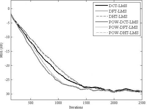
Figure 5. MSE convergence of the TDLMS and the proposed POW-TDLMS for various transforms, N = 16, for AR(1) input signal with ρ = 0.9
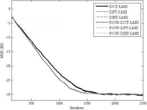
Figure 6. MSE convergence of the TDLMS and the proposed POW-TDLMS for various transforms, N = 16, for AR(1) input signal with ρ = 0.5
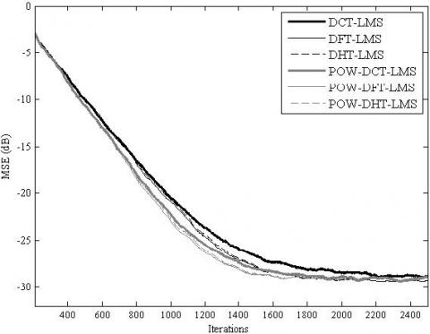
Figure 7. MSE convergence of the TDLMS and the proposed POW-TDLMS for various transforms, N = 64, for AR(1) input signal with ρ = 0.9
Figure 8. MSE convergence of the TDLMS and the proposed POW-TDLMS for various transforms, N = 64, for AR(1) input signal with ρ = 0.5
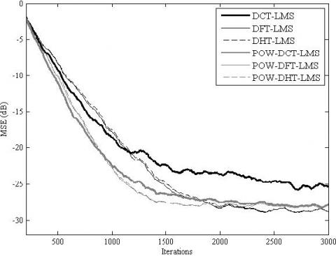
Figure 9. MSE convergence of the TDLMS and the proposed POW-TDLMS for various transforms, N = 128, for AR(1) input signal with ρ = 0.9
The simulation results for the MSE convergence performance are presented in Figure 5, Figure 6, Figure 7, Figure 8, Figure 9 and Figure 10. It is clear from these figures that for all the considered cases, the proposed POW-TDLMS algorithm outperforms the conventional TDLMS algorithm for various transforms in terms of the MSE convergence speed. It is seen from figures 9 and 10 which corresponds to the cases of relatively long filter that the proposed POW-TDLMS algorithm outperforms the conventional TDLMS algorithm for various transforms, especially for the DCT, in terms of the reached steady state.
Figure 10. MSE convergence of the TDLMS and the propo-sed POW-TDLMS for various transforms, N = 128, for AR(1) input signal with ρ = 0.5
In this paper, a new post-whitening transform domain LMS (POW-TDLMS) algorithm has been developed by introducing a first order adaptive post whitening after applying the transform to reinforce its decorrelation. The mean convergence performance analysis of the proposed POW-TDLMS algorithm has also been presented. It has been shown that the proposed POW-TDLMS algorithm significantly reduces the eigenvalue spread of the autocorrelation matrix of the post whitened signal normalized by its power compared to the conventional TDLMS algorithm for the DCT, DFT and DHT transforms. The performance of the proposed POW-TDLMS algorithm has also been evaluated in the context of system identification and in terms of the MSE convergence speed and reached steady state compared to that of the conventional TDLMS algorithm. The obtained results confirm the efficiency and the superiority of the proposed POW-TDLMS algorithm. The proposed algorithm has shown its efficiency in system identification application. Therefore, as a perspective, it would be interesting to investigate its usefulness in adaptive acoustic echo cancellation.
[1] Simon, H. (2002). Adaptive Filter Theory. Prentice-hall. 4rd ed.
[2] Alexander, D.P., Zayed, M.R. (2006). Adaptive filtering primer with matlab. (CRC) Taylor & Francis.
[3] Widrow, B., Hoff, M.E. (1960). Adaptive switching circuits. Tech. Rep. 1553-1, Stanford Electron. Labs., Stanford, CA.
[4] Kim, D.I., Wilde, P.D. (2000). Performance analysis of signed self-orthogonalizing adaptive lattice filter. IEEE transactions on circuits and systems. Analogue and Digital Signal Processing, 47(11): 1227-1237. https://doi.org/10.1109/82.885130
[5] Dimitris, G.M., Vinay, K.I., Stephen, M.K. (2005). Statistical and adaptive signal processing: Spectral estimation, signal modeling. Adaptive Filtering and Array Processing. Artech House.
[6] Homer, J.(2000). Quantifying the convergence speed of LMS adaptive FIR filter with autoregressive inputs. In Electronics Letters, 36(6): 585-586. https://doi.org/10.1049/el:20000469
[7] Mboup, M., Bonnet, M., Bershad, N. (1994). LMS coupled adaptive prediction and system identification: A statistical model and transient mean analysis. IEEE Transactions on Signal Processing, 42(10): 2607-2615. https://doi.org/10.1109/78.324727
[8] Douglas, S.C., Cichocki, A., Amari, S. (1999). Self-whitening algorithms for adaptive equalization and deconvolution. IEEE Transactions on Signal Processing, 47(4): 1161-1165. https://doi.org/10.1109/78.752617
[9] Gazor, S., Lieu, T.(2005). Adaptive filtering with decorrelation for coloured AR environments. IEE Proceedings - Vision, Image and Signal Processing, 152(6): 806-818. https://doi.org/10.1049/ip-vis:20045260
[10] Gonzalez, A., Ferrer, M., Albu, F., Diego, M.D. (2012). Affine projection algorithms: evolution to smart and fast multichannel algorithms and applications. In Proc. of EUSIPCO.
[11] Narayan, S., Peterson, A., Narasimha, M. (1983). Transform domain LMS algorithm. IEEE Transactions on Acoustics, Speech, and Signal Processing, 31(3): 609-615. https://doi.org/10.1109/TASSP.1983.1164121
[12] Lu, J., Qiu X., Zou, H. (2014). A modified frequency-domain block LMS algorithm with guaranteed optimal steady-state performance. Signal Processing, 104: 27-32. https://doi.org/10.1016/j.sigpro.2014.03.029
[13] Chergui, L., Bouguezel, S. (2017). A new pre-whitening transform domain LMS algorithm and its application to speech denoising. Signal Processing, 130: 118-128. http://doi.org/10.1016/j.sigpro.2016.06.021
[14] Boroujeuny, B.F., Gazor, S. (1992). Selection of orthonormal transforms for improving the performance of the transform domain normalised LMS algorithm. IEEE Proceeding F in Radar and Signal Process, 139(5): 327-335. https://doi.org/10.1049/ip-f-2.1992.0046
[15] Lee, K.A., Gan, W.S., Kuo, S.M. (2009). Subband adaptive filtering, theory and implementation. Willey. 1st ed.
[16] Mayyas, K. (2003). New transform domain adaptive algorithms for acoustic echo cancellation. Digital Signal Processing, 13(3): 415-432. https://doi.org/10.1016/S1051-2004(03)00004-6
[17] Shynk, J.J. (1992). Frequency domain and multirate adaptive filtering. IEEE Signal Processing Magazine, 9(1): 14-37. https://doi.org/10.1109/79.109205
[18] Kuhn, E.V., Kolodziej, J.E., Seara, R. (2015). Analysis of the TDLMS algorithm operating in a nonstationary environment. Digital Signal Processing, 45: 69-83. https://doi.org/10.1016/j.dsp.2015.05.013
[19] Zhao, S., Man, Z., Khoo, S., Wu, H.R. (2009). Stability and convergence analysis of transform-domain lms adaptive filters with second-order autoregressive process. IEEE Transactions on Signal Processing, 57(1): 119-130. https://doi.org/10.1109/TSP.2008.2007618
[20] Beaufays, F. (1995). Transform domain adaptive filters: an analytical approach. IEEE Transactions on Signal Processing, 43(2): 422-431. https://doi.org/10.1109/78.348125
[21] Murmu, G., Nath, R. (2011). Convergence performance comparison of transform domain LMS adaptive filters for correlated signal. International Conference on Devices and Communications (ICDeCom), Mesra. https://doi.org/10.1109/ICDECOM.2011.5738534