Abdlmanam S.A. Elmaryami* | Badrul Omar
OPEN ACCESS
The modelling of an axisymmetric industrial quenched chromium steel bar AISI-SAE 5147H, sea water cooled based on finite element method has been produced to investigate the impact of process history on metallurgical and material properties. Mathematical modelling of 1-Dimensional line (radius) element axisymmetric model has been adopted to predict temperature history and consequently the hardness of the quenched steel bar at any point (node). The lowest hardness point (LHP) is determined. In this paper hardness in specimen points was calculated by the conversion of calculated characteristic cooling time for phase transformation t8/5 to hardness. The model can be employed as a guideline to design cooling approach to achieve desired microstructure and mechanical properties such as hardness. The developed mathematical model converted to a computer program. This program can be used independently or incorporated into a temperature history calculator to continuously calculate and display temperature history of the industrial quenched steel bar and thereby calculate LHP. The developed program from the mathematical model has been verified and validated by comparing its hardness results with commercial finite element software results. The comparison indicates reliability of the proposed model.
heat treatment, quenching, axisymmetric chromium steel bar, finite element, mathematical modeling, unsteady state heat transfer
Quenching is a heat treatment usually employed in industrial processes in order to control mechanical properties of steels such as hardness [1]. The process consists of raising the steel temperature above a certain critical value, holding it at that temperature for a specified time and then rapidly cooling it in a suitable medium to room temperature [2]. The resulting microstructures formed from quenching (ferrite, cementite, pearlite, upper bainite, lower bainite and martensite) depend on cooling rate and on chemical composition of the steel [3].
Quenching of steels is a multi-physics process involving a complicated pattern of couplings among heat transfer, because of the complexity, coupled (thermal-mechanical-metallurgical) theory and non- linear nature of the problem, no analytical solution exists; however, numerical solution is possible by finite difference method, finite volume method, and the most popular one - finite element method (FEM) [4]. During the quenching process of the steel bar, the heat transfer is in an unsteady state as there is a variation of temperature with time [5]. The heat transfer analysis in this paper will be carried out in 3- dimensions. The three dimensional analysis will be reduced into a 1-dimensional axisymmetric analysis to save cost and computer time [4, 6-10]. This is achievable because in axisymmetric conditions, there is no temperature variation in the theta Ɵ-direction and in z-direction, the temperature deviations is only in r-direction. The Galerkin weighted residual technique is used to derive the mathematical model. In this paper, 1-Dimensional line (radius) element will be developed.
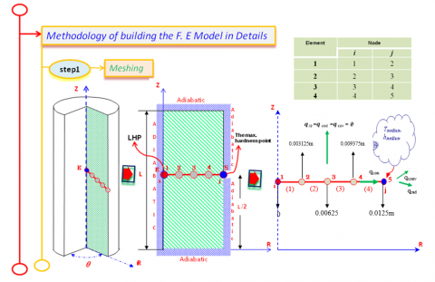
The temperature history of the quenched cylindrical steel bar at any point would like to be calculated; 3-dimensional heat transfer can be analyzed using 1-dimensional axisymmetric elements as shown in Figure 1.
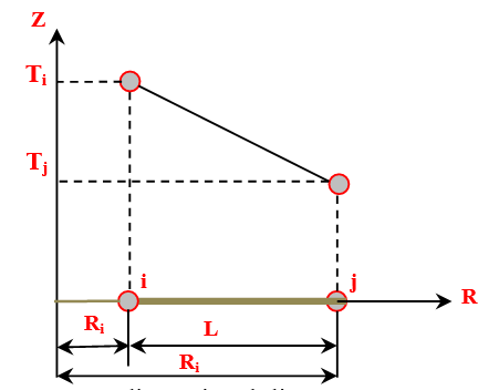
The linear temperature distribution for an element (radius) line, T is given by:
T(R)=a1+a2R (1)
where,
T(R)=nodal temperature as the function of R
a1 and a2 are constants
R is any point on the (radius) line element
2.1 Shape function of the axisymmetric triangular element
The shape functions were to represent the variation of the field variable over the element. The shape function of axisymmetric 1-Dimensional line (radius) element expressed in terms of the r coordinate and its coordinate as shown in Figure 2;
Which are derived to obtain the following shape functions as shown;
${{S}_{i}}=\left( \frac{{{R}_{j}}-R}{{{R}_{j}}-{{R}_{i}}} \right)=\left( \frac{{{R}_{j}}-R}{L} \right)$ (2a)
Figure 1. This figure clearly showed the meshing of axisymmetric one dimensional line (radius) element from the entire domain, the selected 4 elements with 5 nodes and the boundary at node j [5] for an element 4
$\text{Sj}=\left( \frac{R-{{R}_{i}}}{{{R}_{j}}-{{R}_{i}}} \right)=\left( \frac{R-{{R}_{i}}}{L} \right)$ (2b)
Thus the temperature distribution of 1-D radius for an element in terms of the shape function can be written as:
T(R) = SiTi + SjTj = S(r)] {T} (3)
where, [S(r)] = [Si Sj] is a row vector matrix and $\{T\}=\left\{\begin{array}{l}T_{i} \\ T_{j}\end{array}\right\}$ is a column vector of nodal temperature of the element.
Equation (3) can also be expressed in matrix form as:
${{T}_{(R)}}=\left[ {{S}_{i}}\quad {{S}_{i}} \right]\left\{ \begin{array}{*{35}{l}} {{T}_{i}} \\ {{T}_{j}} \\\end{array} \right\}$ (4)
Thus for 1-dimensional element we can write in general:
${{\Psi }_{(e)}}=\left[ \begin{array}{*{35}{l}} {{S}_{i}} & {{S}_{j}} \\\end{array} \right]\left\{ \begin{array}{*{35}{l}} {{\psi }_{i}} \\ {{\psi }_{j}} \\\end{array} \right\}$ (5)
where, Ψi and Ψj represent the nodal values of the unknown variable such as in our case temperature also the unknown can be deflection, or velocity etc.
Figure 2. One-dimensional linear temperature distribution for an element (radius) line in Global Coordinate system
2.2 Natural area coordinate
Using the natural length coordinates and their relationship with the shape function by simplification of the integral of Galerkin solution:
The two length natural coordinates L1 and L2 at any point p inside the element are shown in Figure 3. from which we can write:
$L_{1}=\frac{R_{j}-R}{R_{j}-R_{i}}=\frac{l_{1}}{L}$ (6a)
$L_{2}=\frac{R-R_{i}}{R_{j}-R_{i}}=\frac{l_{2}}{L}$ (6b)
Figure 3. Two-node line element showing interior point p and the two naturals coordinates L1 and L2
Since it is a 1-D element, there should be only one independent coordinate to define any point P. This is true even with natural coordinates as the two natural coordinates L1 and L2 are not independent, but are related as:
$L_{1}+L_{2}=1$ or $L_{1}+L_{2}=\frac{l_{1}}{L}+\frac{l_{2}}{L}=1$ (7)
The natural coordinates L1 and L2 are also the shape functions for the line element, thus:
$S_{i}=\left(\frac{R_{j}-R}{R_{j}-R_{i}}\right)=\left(\frac{R_{j}-R}{L}\right)=L_{1}$ and
$S_{j}=\left(\frac{R-R_{i}}{R_{j}-R_{i}}\right)=\left(\frac{R-R_{i}}{L}\right)=L_{2}$
$S_{i}=L_{1}, S_{j}=L_{2}$ (8)
$R=R_{j} L_{2}+R_{i} L_{1}=R_{i} S_{i}+R_{j} S_{j}$ (9)
$\frac{\partial[S]_{i}}{\partial r}=\frac{\partial L_{1}}{\partial r}=\frac{-1}{R_{j}-R_{i}}=-\frac{1}{L}$ (10)
$\frac{\partial[S]_{j}}{\partial r}=\frac{\partial L_{2}}{\partial r}=\frac{1}{R_{j}-R_{i}}=\frac{1}{L}$ (11)
2.3 Develop equation for all elements of the domain
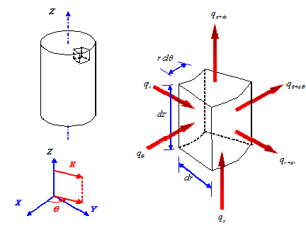
Derivation of equation of heat transfer in axisymmetric 1-D line (radius) elements by applying the conservation of energy to a differential volume cylindrical segment as shown in Figure 4;
Figure 4. Axisymmetric element from an axisymmetric body
Ein – Eout + Egenerated = Estored (12)
The transient heat transfer within the component during quenching can mathematically be described by simplifying the differential volume term; the heat conduction equation is derived and given by;
$\frac{1}{r} \frac{d}{d r}\left(k_{r} r \frac{d T}{d r}\right)+\frac{1}{r^{2}} \frac{d}{d \theta}\left(k_{\theta} \frac{d T}{d \theta}\right)+\frac{d}{d z}\left(k_{z} \frac{d T}{d z}\right)+q=\rho c \frac{d T}{d t}$ (13)
kr = heat conductivity coefficient in r-direction, W/m∙°C.
kθ = heat conductivity coefficient in θ-direction, W/m∙°C.
kz = heat conductivity coefficient in z-direction, W/m∙°C.
T = temperature, °C.
q = heat generation, W/m3.
ρ = mass density, kg/m3.
c = specific heat of the medium, J/kg∙K.
t = time, s.
2.4 The assumption made in this problem was
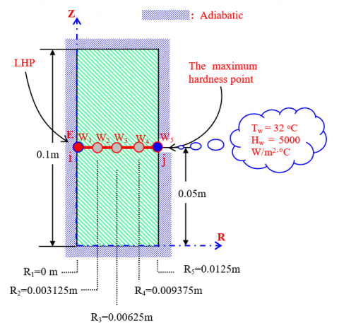
(1) For axisymmetric situations 1-D line (radius) element, there is no variation of temperature in the Z-direction as shown in Figure 1, because we already assumed that in steel quenching and cooling process of the steel bar is insulated from convection at the cross section of the front and back. It means that we have convection and radiation at one node only which is on the surface [node 5], in our research we focus to calculate LHP which is at [node 1], where it is the last point will be cooled, this give the maximum advantage to make our assumption more safe, because it is the last point which will effect by convection and radiation from the front and back cross section of the steel bar therefore we can write, $\left(\frac{\partial T}{\partial z}=0\right)$.
(2) For axisymmetric situations, there is no variation of temperature in the θ-direction, because it is clear from Figure 1 that the temperature distribution along the radius will be the same if the radius move with angle θ, 360o therefore, $\left(\frac{\partial T}{\partial \theta}=0\right)$.
(3) The thermal energy generation rate(Ý) represent the rate of the conversion of energy from electrical, chemical, nuclear, or electromagnetic forms to thermal energy within the volume of the system. Such as conversion is the electric field which will be studied with details in the 2nd part of our research, however in this manuscript no heat generation therefore, $\mid \dot{q}=0$
After simplifying, the Eq. (13) become;
$\frac{k}{r} \frac{\partial}{\partial r}\left(r \frac{\partial T}{\partial r}\right)=\rho c \frac{\partial T}{\partial t}$ (14)
And also known as residual or partial differential equation
$\{\Re\}=\frac{k}{r} \frac{\partial}{\partial r}\left(r \frac{\partial T}{\partial r}\right)-\rho c \frac{\partial T}{\partial t}=0$ (15)
2.5 Galerkin weighted residual method formulation
From the derived heat conduction equation, the Galerkin residual for 1-Dimensional line (radius) element in an unsteady state heat transfer by integration the shape functions times the residual which minimize the residual to zero becomes;
$\int_{V}[S]^{T}\{\Re\}^{(e)} d v=0$ (16)
where, [S]T = the transpose of the shape function matrix
$\{\mathfrak{R}\}_{(e)}$= the residual contributed by element (e) to the final system of equations.
$\frac{k}{r} \int[S]^{T} \frac{\partial}{\partial r}\left(r \frac{\partial T}{\partial r}\right) d v-\int[S]^{T} \rho c \frac{\partial T}{\partial t} d v=0$ (17)
2.6 Chain rule
The term 1 and 2 of Eq. (17) can be re-arranged using the chain rule which states that;
$(f g)^{-}=f g^{-}+g f^{-}$
Therefore, $f g^{-}=(f g)^{-}-f^{-} g$ then $\frac{\partial}{\partial r}\left([S]^{T} r \frac{\partial T}{\partial r}\right)=$ $[S]^{T}\left\{\frac{\partial}{\partial r}\left(r \frac{\partial T}{\partial r}\right)\right\}+r \frac{\partial T}{\partial r} \frac{\partial[S]^{T}}{\partial r}$
Term 1 of Eq. (17) is rearranged thus;
$[S]^{T}\left\{\frac{\partial}{\partial r}\left(r \frac{\partial T}{\partial r}\right)\right\}=$$\frac{\partial}{\partial r}\left([S]^{T} r \frac{\partial T}{\partial r}\right)-r \frac{\partial T}{\partial r} \frac{\partial[S]^{T}}{\partial r}$ (18)
By substitute Eq. (18) in to Eq. (17), get
$\begin{align} & =\overbrace{\frac{k}{r}\int{\left\{ \frac{\partial }{\partial r}\left( {{\left[ S \right]}^{T}}r\frac{\partial T}{\partial r} \right) \right\}dv}}^{A}- \\ & \overbrace{\frac{k}{r}\int{\left\{ \frac{\partial {{\left[ S \right]}^{T}}}{\partial r}r\frac{\partial T}{\partial r} \right\}dv}}^{B}-\underbrace{\int{{{\left[ S \right]}^{T}}\left\{ {{\rho }_{{}}}{{c}_{{}}}\frac{\partial T}{\partial t} \right\}dv}}_{C} \\ \end{align}$ (19)
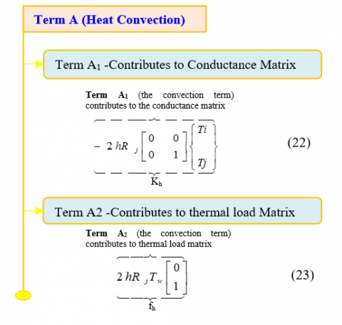
Term A is the heat Convection Terms and contributes to the Conductance and Thermal Load Matrix. Term B is the Heat Conduction Terms and contributes to the Conductance Matrix. Term C is the transient equation and contributes to the Capacitance Matrix.
where,
$\begin{align} & \overbrace{\frac{k}{r}\int{\left\{ \frac{\partial }{\partial r}\left( {{\left[ S \right]}^{T}}r\frac{\partial T}{\partial r} \right) \right\}dv}}^{A}= \\ & \underbrace{-2\pi hrz{{\left[ S \right]}^{T}}\left[ S \right]{{\left\{ T \right\}}^{e}}}_{(1)}+\underbrace{2\pi hrz{{\left[ S \right]}^{T}}{{T}_{f}}}_{(2)}- \\ & \underbrace{2\pi rz{{\varepsilon }_{s}}\sigma {{\left[ S \right]}^{T}}\left[ S \right]{{\left\{ T \right\}}^{e}}{{\left( \left[ S \right]{{\left\{ T \right\}}^{e}} \right)}^{3}}}_{(3)}+\underbrace{2\pi rz{{\varepsilon }_{s}}\sigma {{\left[ S \right]}^{T}}T_{f}^{4}}_{(4)} \\ \end{align}$
Note: term (1) and term (3) contributed to the conductance matrix since they contains the unknown temperature {T}. Term (2) and (4) contributed to the thermal load matrix as Tf is the known fluid temperature. Term (3) and term (4) heat radiation very important if our heat treatment is Annealling [cooling in the furnace] or Normalizing [cooling in air or jet air], but can be ignore if the cooling is quenching in sea water as in our work.
From earlier explanations derivation and after simplification we can formulate the conductance matrix in the r-direction for term B finally we get:
Term B (the conduction term) contributes to the conductance matrix
Similarly, Term C, the unsteady state (transient) which contributes to the Capacitance Matrix becomes:
Term C (heat stored) contributes to the Capacitance Matrix
$\underbrace{\overbrace{\frac{k}{L}\left( {{R}_{j}}+{{R}_{i}} \right)\left[ \begin{matrix} 1 & -1 \\ -1 & 1 \\\end{matrix} \right]\left\{ \begin{matrix} Ti \\ {} \\ Tj \\\end{matrix} \right\}}^{{}}}_{{}}$ (20)
$\underbrace{\overbrace{\frac{L\rho c}{6}\left[ \begin{matrix} \left( 3{{R}_{i}}+{{R}_{j}} \right) & \left( {{R}_{i}}+{{R}_{j}} \right) \\ \left( {{R}_{i}}+{{R}_{j}} \right) & \left( {{R}_{i}}+3{{R}_{j}} \right) \\\end{matrix} \right]\left\{ \begin{matrix} {{{\dot{T}}}_{i}} \\ {} \\ {{{\dot{T}}}_{j}} \\\end{matrix} \right\}}^{{}}}_{{}}$ (21)
2.7 Construct the element Matrices to the Global Matrix
The global, conductance, capacitance and thermal load matrices and the global of the unknown temperature matrix for all the elements in the domain are assembled i.e. the element's conductance, capacitance and thermal load matrices have been derived. Assembling these elements is necessary in all finite element analysis [11-13].
Constructing these elements will result into the following finite element equation:
$[K]^{(G)}\{T\}^{(G)}+[C]^{(G)}\{\dot{T}\}^{(G)}=\{F\}^{(G)}$ (24)
where:
$[K]=\left[K_{c}\right]+\left[K_{h}\right]$: is conductance matrix due to Conduction (Elements 1 to 4) and heat loss through convection at the element’s boundary (element 4 node 5) as shown in Figure 1.
{T}: is temperature value at each node, °C.
[C]: is capacitance matrix, due to transient equation (heat stored)
$\{ \dot{T}\}$: is temperature rate for each node, °C/s.
$\{F\}=\left\{F_{h}\right\}+\left\{F_{\dot{q}}\right\}$: is heat load due to heat loss through convection at the element’s boundary (element 4 node 5) and internal heat generation (element 4 node 5).
2.8 Euler’s method
Two point recurrence formulas will allow us to compute the nodal temperatures as a function of time. In this paper, Euler’s method which is known as the backward difference scheme (FDS) will be used to determine the rate of change in temperature, the temperature history at any point (node) of the steel bar [5, 14-17].
If the derivative of T with respect to time t is written in the backward direction and if the time step is not equal to zero (Dt¹0), we have;
$\{ \dot{T}\} \approx\left\{\frac{T(t)-T(t-\Delta t)}{\Delta t}\right\}$ (25)
With;
$\dot{T}=$ temperature rate (°C/s); T(t)= temperature at t s (°C); T(t-Dt)=temperature at (t-Dt) s, (°C)
Dt = selected time step (s) and t=time (s) (at starting time, t-0)
By substituting the value of $\{\dot{T}\}$ into the finite element global equation, we have that;
$[K]^{(G)}\{T(t)\}^{(G)}+$$[C]^{(G)}\left\{\frac{T(t)-T(t-\Delta t)}{\Delta t}\right\}^{(G)}=\{F(t)\}^{(G)}$ (26)
$\left[[K]^{(G)} \Delta t+[C]^{(G)}\right]\{T\}_{i+1}^{(G)}=$$[C]^{(G)}\{T\}_{i}^{(G)}+\{F\}_{i+1}^{(G)} \Delta t$ (27)
From Eq. (27) all the right hand side is completely known at time t, including t = 0 for which the initial condition apply.
Therefore, the nodal temperature can be obtained for a subsequent time given the temperature for the preceding time.
Once the temperature history is known the important mechanical properties of the chromium steel bar can be obtained such as hardness and strength.
3.1 Calculation the temperature history
The present developed mathematical model is programmed using MATLAB to simulate the results of the temperature distribution with respect to time in transient state heat transfer of the industrial quenched chromium steel bar. The cylindrical chromium steel bar has been heated to 850°C. Then being quenched in sea water with Tsea-water = 32°C and convection heat transfer coefficient, hsea-water = 1250 W/m2∙°C [18]. The temperature history for the selected nodes of the cylindrical chromium steel bar after quenching is being identified in Figure 5 and Figure 6. The cylindrical bar was made from chromium steel 5147H, with properties as mentioned below [8-10, 18, 19].
Thermal capacity, ρc (J/m3∙°C)
$0 \leq T \leq 650^{\circ} \mathrm{C}, \rho c=(0.004 \quad T+3.3) \times 10^{6}$
$650 \quad<T \leq 725^{\circ} \mathrm{C}, \rho c=(0.068 \quad T-38.3) \times 10^{6}$
$725<T \leq 800^{\circ} \mathrm{C}, \rho c=(-0.086 \quad T+73.55) \times 10^{6}$
$T>800^{\circ} \mathrm{C}, \rho c=9.55 \times 10^{6}$
Thermal conductivity, k (W/m∙°C)
$0 \leq T \leq 900^{\circ} \mathrm{C}, k=-0.022$
$T+48, T>900^{\circ} \mathrm{C}, k=28.4$
In our case Eq. (27) becomes;
$[K]^{(G)}\{T\}^{(G)}+[C]^{(G)}\{\dot{T}\}^{(G)}=\{F\}^{(G)}$
And their respective equation;
$[K]^{(G)}=\left[K_{c}\right]^{(1)}+\left[K_{c}\right]^{(2)}+\left[K_{c}\right]^{(3)}+\left[K_{c}\right]^{(4)}+\left[K_{h}\right]^{(4)}$ (28)
$[C]^{(G)}=[C]^{(1)}+[C]^{(2)}+[C]^{(3)}+[C]^{(4)}$ (29)
$\{F\}^{(G)}=\left\{F_{h}\right\}^{(4)}$ (30)
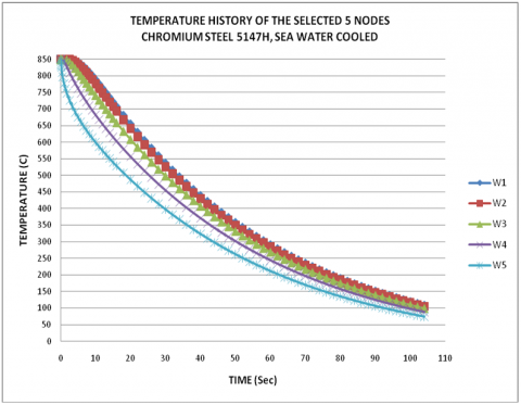
With the input data and boundary conditions provided, a sensitivity analysis is carried out with the developed program to obtain the temperature distribution at any point (node) of the quenched chromium steel bar. As an example, the transient state temperature distribution results of the selected five nodes from the center [W1] to the surface [W5] of the quenched steed bar which were computed are shown in Figure 5 and Figure 6.
Figure 5. The axisymmetric one dimensional line (radius) element from the domain when the radius equal 12.5mm, the selected 4 elements with 5 nodes and the boundary at node j [2] for an element 4
Figure 6. Graph of temperature history along WW cross-section from MATLAB program
3.2 LHP Calculation
3.2.1 Calculating the cooling time required
In this study, we choose to calculate the cooling time between 800oC and 500oC [14, 20-26]. Where, the characteristic cooling time, relevant for phase transformation in most structural steels is the time of cooling from 800 to 500°C (time t8/5) [7, 11-13, 27-29, 30].
tc= t800-t500
From Figure 6 we can determine the time taken for node W1 to reach 800oC,
t800°C=9.216 sec.
By the same way the time taken for node W1 to reach 500oC is t500°C=33.639 sec.
So the Cooling time tc for node W1;
tc=t500°C-t800°C=33.639–9.216 = 24.423 sec
For nodes W2 to W5, the cooling time tc calculated by the same way, the final results shown in Table 1.
3.2.2 Calculating the Jominy distance from Standard Jominy distance versus cooling time curve
Cooling time, tc obtained will now be substituted into the Jominy distance versus cooling time curve to get the correspondent Jominy distance. Jominy distance can also be calculated by using polynomial expressions via polynomial regression via Microsoft Excel.
In this paper the standard Table [30] will be used. Then Jominy distance of nodes W1 to W5 will be calculated by using the data from [30], the final results shown in Table 1, where the Rate of Cooling, ROC, was defined by;
$R O C=\frac{800^{\circ} \mathrm{C}-500^{\circ} \mathrm{C}}{t_{c}}=\frac{800^{\circ} \mathrm{C}-500^{\circ} \mathrm{C}}{t_{500^{\circ} \mathrm{C}}-t_{800^{\circ} \mathrm{C}}}\left({ }^{\circ} \mathrm{C} / \mathrm{s}\right)$
3.2.3 Predict the hardness of the quenched steel bar
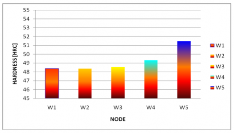
Figure 7. Hardness distribution along WW cross section for the nodes W1 to W5 from the centre to the surface respectively at half the length at the centre of the quenched steel bar
Table 1. Cooling time, Cooling rate, Jominy distance and HRC for the nodes W1 to W5, sea water cooled
|
Node |
tc (s) |
ROC (°C /s) |
Jominy-distance (mm) |
Hardness HRC) |
|
W1 |
24.423 |
12.2835 |
15.594 |
48.360 |
|
W2 |
24.369 |
12.3107 |
15.574 |
48.385 |
|
W3 |
23.961 |
12.5203 |
15.426 |
48.571 |
|
W4 |
22.295 |
13.4559 |
14.821 |
49.332 |
|
W5 |
18.194 |
16.4889 |
13.345 |
51.486 |
The HRC of chromium steel AISI-SAE 5147H can be calculated by using the relation between the J-Distance and the HRC from the Practical date Handbook, the Timken Company 1835 Duebex Avenue SW Canton, Ohio 44706-2798 1-800-223, the final results shown in Figure 7 and Table 1.
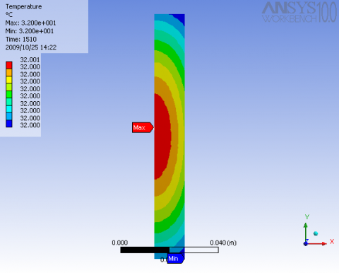
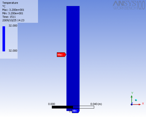
The same data input for the steel properties and boundary condition used in the mathematical model is applied to the ANSYS software to verify the temperature simulation results. The temperature distribution from the ANSYS analysis is depicted figuratively as shown in Figure 8a and Figure 8b;
Figure 8a. The temperature distribution just before the steel bar becomes completely cooled
Figure 8b. The temperature distribution at the moment that the entire steel bar becomes completely cooled after 1511s
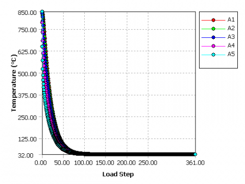
The temperature time graph from the ANSYS analysis is depicted as shown in Figure 9;
From the graphs shown in Figure 6 by mathematical model and Figure 9 by ANSYS, it can be clearly seen that the temperature history of the quenched steel bar have the same pattern. The heat transfer across the steel bar is uniform. From Figure 7 the cooling time, Jominy-distance and consequently the hardness of the quenched chromium steel 5147H at any point (node), even the lowest hardness point (LHP) is determined by ANSYS too, the final results shown in Table 2 and Figure 10.
Figure 9. Temperature-time graph from ANSYS
Table 2. Cooling time, Cooling rate, Jominy distance and HRC for the nodes A1 to A5, sea water cooled by ANSYS
|
Node |
Cooling time, |
Cooling rate |
J-distance (mm) |
HRC |
|
A1 |
32.596854 |
9.20334 |
18.937 |
46.071 |
|
A2 |
32.519782 |
9.22515 |
18.913 |
46.086 |
|
A3 |
31.558004 |
9.50630 |
18.618 |
46.272 |
|
A4 |
29.663021 |
10.1136 |
18.038 |
46.636 |
|
A5 |
23.618155 |
12.7020 |
15.302 |
48.357 |
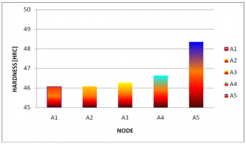
Figure 10. Hardness distribution by ANSYS along AA cross section for the nodes A1 to A5 from the centre to the surface respectively at half the length at the centre of the quenched steel bar
From our results we found that in the mathematical model for the 1st node with W1 in the center, we found that HRC=48.360. While in ANSYS for the same node A1, we found that HRC=46.071. And for the nodes on the surfaces W5 and A5, it was found that HRC=51.486 and 48.357 for the mathematical model and ANSYS respectively. From the above, it can be seen that there is a strong agreement between both results. The difference between all the results of the mathematical model and the ANSYS simulations can be accounted due to the fact that the ANSYS software is commercial purpose, and thereby has some automated input data. But the developed mathematical model is precisely for a circular steel bar axisymmetric cross section.
However, there is strong agreement between both results and thereby the result is validated where, the comparison indicated reliability of the proposed model. Also the results showed that the node on the surface will be the 1st which completely cooled after quenching because it is in the contact with the cooling medium then the other nodes on the radial axis to the centre respectively and the last point will be completely cooled after quenching will be at half the length at the centre. Hence LHP will be at half the length at the centre of the quenched industrial chromium steel bar. It will be more important to know LHP once the radius of the quenched steel bar is large because LHP will be low, in other words will be lower than the hardness on the surface, that means increasing the radius of the bar inversely proportional with LHP.
LHP calculation experimentally is an almost impossible task using manual calculation techniques also the earlier methods only used hardness calculated at the surface, which is higher than LHP, this has negative consequence which can result to the deformation and failure of the component.
A mathematical model of steel quenching has been developed to compute LHP of the quenched chromium steel 5147H at any point (node) in a specimen with cylindrical geometry. The model is based on the finite element Galerkin residual method. The numerical simulation of quenching consisted of numerical simulation of temperature transient field of cooling process. This mathematical model was verified and validated by comparing the hardness results with ANSYS software simulations. From the mathematical model and ANSYS results, it is clear that the nodes on the surface [W5 and A5] respectively cools faster than the nodes on the center [W1 and A1] because tCW5 less than tCW1 and tCA5 less than tCA1, this means that the mechanical properties will be different such as hardness where the hardness on the surface nodes [W5 and A5] will be higher than the hardness on the center nodes [W1 and A1].
The authors would like to thank {Ministry of Science, Technology and Innovation, Malaysia} for supporting this research under the Science Fund Grant with grant number {03-01-13-SF0071}.
The corresponding author is grateful to the Bright Star University [BSU], El-Brega - Libya for supporting this Paper.
[1] Smoljan, B. (2003). Inverse hardness distribution in quenched steel specimen of complex form. In Proceedings of the 12th Scientific International Conference on “Achievements in Mechanical and Materials Engineering”, pp. 817-820.
[2] Elmaryami, A.S., Omar, B. (2012). Unsteady State computer simulation of 2 chromiumsteel at 925 degrees c as austenitizing temperature to determine the lowest hardness point (LHP). Metallurgical & Materials Engineering, 18(2): 79-91.
[3] Elmaryami, A.S., Omar, B. (2012). Developing 1-dimensional transient heat transfer axi-symmetric MM to predict the hardness, determination LHP and to study the effect of radius on E-LHP of industrial quenched steel bar. Heat Transfer Phenomena and Applications, 153-182. https://doi.org/10.5772/51947
[4] Robert, K.N. (2001). Quenching and tempering of welded steel tubular. July, 29, 2001. The FABRICATOR articles.
[5] Elmaryami, A.S., Omar, B. (2012). Modeling the lowest hardness point in a steel bar during quenching. Materials Performance and Characterization, 1(1): 1-15. https://doi.org/10.1520/MPC104386
[6] Elmaryami, A.S., Omar, B. (2012). Determination LHP of axisymmetric transient Molybdenum steel-4037H quenched in sea water by developing 1-d mathematical model. Metallurgical and Materials Engineering, 18(3): 203-222.
[7] Elmaryami, A.S., Omar, B. (2013). Effect of radius on temperature history of transient industrial quenched chromium Steel-8650H by developing 1-D MM. Applied Mathematical Sciences, 7(10): 471-486. https://doi.org/10.12988/ams.2013.13041
[8] Elmaryami, A.S.A., Sousi, A., Saleh, W., El-Mabrouk Abd El-Mawla, S., Elshayb, M. (2019). Maximum allowable thermal stress calculation of water tube boiler during operation. International Journal of Research - Granthaalayah, 7(7): 191-199. https://doi.org/10.5281/zenodo.3358065
[9] Elmaryami, A.S., Omar, B. (2012). Modeling LHP in carbon steel-1045 during quenching. Journal of Mathematical Theory and Modeling, 2(12): 35-47.
[10] Elmaryami, A.S., Omar, B. (2011). International Conference on Management and Service Science, MASS, Wuhan, China, Article number 5999335, 2011. Indexed by Ei Compendex, Sponsors: IEEE. SCOPUS indexed.
[11] Elmaryami, A.S., Omar, B.B. (2011). The lowest hardness point calculation by transient computer simulation of industrial steel bar quenched in oil at different austenitizing temperatures. In 2011 International Conference on Management and Service Science, pp. 1-6. https://doi.org/10.1109/ICMSS.2011.5999335
[12] Elmaryami, A.S.A. (2008). Materials Science and Technology Conference and Exhibition, MS&T'08. Pittsburgh, PA; United States, 2008: 1502-1514.
[13] Mittemeijer, E.J. (2013). Steel Heat treating Fundamentals and Processes. ASM Handbook A, 4: 2013. https://doi.org/10.31399/asm.hb.v04a.9781627081658
[14] Elmaryami, A.S.A., Elshayeb, M., Omar, H.B.B., Basu, P., Hasan, S.B.H. (2013). Development of a numerical model of quenching of steel bars for determining cooling curves. Metal Science and Heat Treatment, 55(3-4): 216-219. https://doi.org/10.1007/s11041-013-9608-6
[15] Omar, B., Elmaryami, A.S. (2013). Developing 1-D MM of transient industrial quenched chromium steel-5147H to study the effect of radius on temperature history. In Advanced Materials Research, 711: 115-127. https://doi.org/10.4028/www.scientific.net/AMR.711.115
[16] Elmaryami, A.S., Omar, B. (2012). Developing 1D MM of axisymmetric transient quenched chromium steel to determine LHP. Journal of Metallurgy, 2012: 539823. https://doi.org/10.1155/2012/539823
[17] Elmaryami, A.S., Omar, B. (2011). Developing 1-D mm of axisymmetric transient quenched molybdenum steel AISI-SAE 4037H to determine lowest hardness point. Journal of Metallurgy and Materials Science, 53(3): 289-303.
[18] Elmaryami, A.S., Omar, B. (2012). Modeling LHP in carbon steel-1045 during quenching. Journal of Mathematical Theory and Modeling, 2(12): 35-47.
[19] Elmaryami, A.S., Omar, B. (2011). Transient computer simulation of industrial quenched steel bar to determine LHP of molybdenum and boron steel at 850 C as austenitizing temperature quenched in different medium. International Journal of Material Science, 8(1): 13-28.
[20] Omar, B., Elshayeb, M., Elmaryami, A.S.A. (2009). 18th World IMACS Congress and MODSIM09 International Congress on Modelling and Simulation: Interfacing Modelling and Simulation with Mathematical and Computational Sciences, MODSIM09; Cairns, QLD; 1699-1705.
[21] Elmaryami, A.S.A., Hasan, S.B.H., Omar, B., Elshayeb, M. (2009). Materials Science and Technology Conference and Exhibition, (MS & T'09), David L. Lawrence Convention Centre, Pittsburgh, Pennsylvania, USA, 3: 1514-1520.
[22] Moaveni, S. (2011). Finite element analysis theory and application with ANSYS, 3/e. Pearson Education India.
[23] Mohamed, E., Bing, Y.K. (2000). Application of finite difference and finite element methods. University Malaysia Sabah Kota Kinabalu. 2000.
[24] Smoljan, B. (2005). Mathematical modelling of austenite decomposition during the quenching. In Proceedings of 13th International Scientific Conference AMME, pp. 593-596.
[25] Smoljan, B. (2006). Prediction of mechanical properties and microstructure distribution of quenched and tempered steel shaft. Journal of Materials Processing Technology, 175(1-3): 393-397. https://doi.org/10.1016/j.jmatprotec.2005.04.068
[26] Smoljan, B., Iljkić, D., Hanza, S.S. (2009). Computer simulation of working stress of heat treated steel specimen. Journal of Achievements in Materials and Manufacturing Engineering, 34(2): 152-156.
[27] Moaveni, S. (2003). Finite Element Analysis. A Brief History of the Finite Element Method and ANSYS. 6-8. Pearson Education, 2003, Inc.
[28] Elmaryami, A.S. (2017). Abd-Allah Alsoussi, Mohammad Gomaa, and Elssamoussi Abd-Allah., “Determination the cooling time, rate of cooling, jominy distance and the hardness during heat transfer of quenched steel bar”. Journal of Science-Garyounis University, 38(5): 0-11.
[29] Elmaryami, A.S., Omar, B. (2013). Modeling the effect of radius on temperature history of transient quenched boron steel. Acta Metallurgica Slovaca, 19(2): 105-111. http://dx.doi.org/10.12776/ams.v19i2.94
[30] Chandler, H. (1999). Hardness testing. ASM international. Hardness Testing Second Edition: 111-133. United States of America: ASM International.