Gianluca Coccia* | Alice Mugnini | Fabio Polonara | Alessia Arteconi
OPEN ACCESS
When used to model buildings in model predictive controls (MPCs), artificial neural networks (ANNs) have the advantage of not requiring a physical model of the building, thus simplifying the development of the MPC. However, if the MPC is intended to operate on the HVAC control system of the building to unlock its energy flexibility, some specific issues associated to the use of ANNs could arise. Thus, in this work we give an insight on the use of ANNs in MPCs, focusing our analysis on some of the most relevant ANN architectures that can be used to predict the thermal demand of a building. Furthermore, the integration of MPCs in real buildings, along with the possibility to unlock energy flexibility by intervening on the comfort band, are discussed. Some issues related to the use of ANN-based MPCs combined with the activation of energy flexibility (e.g., difficulty in training the ANN or in managing flexibility by the MPC) are also investigated.
ANN, MPC, energy flexibility, building model
In the building sector, the possibility to use advanced controls such as model predictive controls (MPCs) allows to improve energy management and reduce the consumption of primary energy [1]. MPCs are based on dynamic models that allow to forecast the energy behavior of a building [2, 3]; in this way, an MPC is able to select proper control actions and decisions that can hinder future disturbances, while maintaining the system constraints [4].
Among the possibilities given by the use of MPCs in buildings, it should be mentioned the optimized integration with renewable energy sources (RESs) or energy storages, and in particular thermal energy storages (TESs). But MPCs could also be used to unlock the energy flexibility of a building. In buildings, energy flexibility can be referred to as a static or dynamic function suitable for control [5]. Buildings have the opportunity to activate their energy flexibility in two main ways: by using their thermal mass or insulation, or by operating on their HVAC (Heating, Ventilation and Air-Conditioning) system. The latter flexibility mode can be unlocked by allowing the indoor temperature to vary in a wider comfort range, which is regulated on the basis of price signals. Based on this assumption, it is evident that if the HVAC system is managed by an MPC, then there should be the chance to enhance the flexibility unlocking, i.e. to improve and optimize the load shifting potential.
In order to establish an optimal control strategy, an MPC is supposed to operate on an accurate representation of the building to be controlled [6]. According to the paradigm followed to model the building, it is possible to distinguish between white [7], grey [8], or black box models [9]. White box models (also defined physical-based models) are accurate representations of the building being examined, and thus require a detailed formulation of the building physical and thermal properties by means of energy and mass conservation equations. Their complexity is counterbalanced by the fact that they do not need training data in order to be developed.
To reduce the complexity of white box models, grey box (or hybrid) models combine a partial theoretical structure, usually written in a parametric form, with training data that integrate the model itself. Given their hybrid nature, not all the internal parameters and equations can be therefore interpreted under a physical point of view.
Black box models (or data-driven models), instead, are a pure mathematical formulation of the building, thus they do not require a physical knowledge of the building. Differently from white box models, however, data-driven models need to be trained with a large amount of data collected over a proper period, and such data are required to be statistically representative of the operation of the building under study.
Over the last years, a category of black box models that has received lots of attention by researchers is that comprising artificial neural networks (ANNs). The structure of ANNs is inspired to that of a biological brain, i.e. the inputs of an ANN correspond to the dendrites of a biological brain, while the outputs of an ANN can be imagined as the axons of the same brain. The processing of the inputs takes place in the neurons, in the same fashion of a biological brain; neurons apply a nonlinear activation function on the input data and provide the corresponding outputs. Considering the possibilities offered by data mining, machine learning and big data [10], MPCs using a building model based on ANNs are expected to improve both prediction capability and overall efficiency of residential systems.
Analyzing the literature associated to the use of ANN-based MPCs in building, and to the activation of energy flexibility, it is possible to assess that a number of interesting papers has been published. For instance, in the work by Ferreira et al. [11] a discrete MPC using an ANN with a radial basis function architecture is proposed. The model is validated with experimental results carried out in a building of University of Algarve. According to the authors, the use of the ANN-based MPC allows to reach energy savings greater than 50%. In the paper by Ruano et al. [12], the authors discuss the development of an ANN-based MPC used to manage the HVAC system of a University building. Compared to standard temperature-regulated controls, the ANN-based MPC seems to provide results similar to those provided by Ferreira et al. [11]. Afram and Janabi-Sharifi [13] propose a supervisory controller based on an MPC to shift the heating and cooling loads of a residential building to off-peak hours. Analyzing the experimental results determined in a house used as case study, the authors show that the flexibility provided by the MPC allows to obtain a 16% cost saving compared to the use of standard controls based on fixed setpoints. In a review written by the same authors [14], another case study is evaluated, and it is assessed that cost savings from 6% to 73% can be achieved by controlling an HVAC system with an ANN-based MPC rather than by using standard thermostats. In the work by Mugnini et al. [15], an operative MPC is tested with two different building models: a physical-model based on a resistance-capacitance network, and a data-driven model based on an ANN. Although both models ensure an energy cost saving of about 16%, their behavior when actually implemented in the HVAC control system of the building is different; specifically, the physical-based model seems to follow the thermal dynamics of the building better than the ANN model, which shows some issues when energy flexibility is activated.
The analysis of the literature reveals that ANN-based MPCs used in buildings have been studied in detail. However, according to the authors of the present work, there are two important aspects that have not been discussed in detail: a) the rise of issues associated to the use and training of ANNs in MPCs and b) the effects derived by unlocking energy flexibility when such MPCs are actually used in real buildings. Given the relevance that the two aspects could have on the performance of an MPC used in buildings, in this paper they will be discussed in detail and some recommendations will be provided in order to improve the prediction capability of an MPC using an ANN as building model.
The paper is structured as follows. Section 2 describes some architectures of ANNs that could be used to simulate the thermal demand of a building, and their advantages and disadvantages when implemented in actual MPCs. Section 3 depicts how energy flexibility can be unlocked in buildings when the HVAC system is being controlled by an ANN-based MPC. Section 4 highlights the issues that can occur when an ANN-based MPC is used to manage energy demand in a building. Finally, Section 5 reports the conclusions of the work.
When an MPC is based on an ANN to predict the thermal demand of a building, it is fundamental having the availability of a relevant amount of training data that can be used to define the ANN itself. Before training, however, it is important selecting the proper architecture of ANN that represents the energy behavior of the building under study. The scope of the next subsections is therefore to provide some useful information about the typical ANN architectures that can be used as building model. Before examining in more detail such architectures, however, some general aspects related to the training and functioning of ANNs will be discussed first.
2.1 Training of ANNs
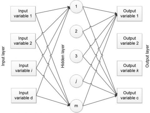
As highlighted in the introduction, artificial neural networks (ANNs) are mathematical models that reflect the functioning of a biological brain [16]. The inputs of the network (x) are processed by neurons, which apply a nonlinear activation function, g, and give the outputs of the network (y). Let us consider a feedforward multilayer perceptron ANN, consisting of one input layer, one output layer, and only one layer of neurons. This layer is usually referred to as hidden layer, because its activation values are not directly accessible from outside the network [16]. If the activation function in the output layer is defined by a function h, in general different from g, the mapping carried out by the ANN on the input layer can be written as:
$y_{k}=\mathrm{h}\left(\sum_{j=0}^{\mathrm{m}} w_{k j}^{\prime \prime} \mathrm{g}\left(\sum_{i=0}^{\mathrm{d}} w_{j i}^{\prime} x_{i}\right)\right)$ (1)
where, d denotes the number of inputs of the ANN, w’ji is the weight and bias matrix of the inputs, m is the number of neurons in the hidden layer, and w’’kj is the weight and bias matrix of the hidden layer. An example of ANN based on a feedforward multilayer perceptron architecture is depicted in Figure 1.
Figure 1. ANN with a feedforward multilayer perceptron architecture
Since ANNs are pure mathematical models with no physical meaning, they need to be trained with a set of available data. The objective of the training consists in determining the parameters that actually define an ANN, i.e. its weight and bias coefficients. Let us then consider a training dataset defined by an input vector xq = (x1q, …, xdq), where d denotes the number of inputs of the ANN and q = 1, …, n is an index indicating a particular point of each input. Each input vector xq has a corresponding target vector tq = (t1q, …, tcq), which represents the desired values for the output yk (k = 1, …, c is the number of outputs in the ANN). In order to find suitable values for the weights and biases of the ANN, a good indicator is the square error between the desired target value tqk and the corresponding value predicted by the ANN through the output yk, which is a function of xq and w, the vector of weights and biases. If the square error is summed over all datapoints, it is possible to write:
$E=\frac{1}{2} \sum_{a=1}^{n} \sum_{k=1}^{c}\left(y_{k}\left(x^{q}, \mathbf{w}\right)-t_{k}^{q}\right)^{2}$ (2)
Eq. (2) represents the error function used in the training of the ANN. As can be noted, E is a function of the vector of weights and biases, w, so it can be fitted to the training data by selecting a value of w that minimizes E. The minimization of E can be carried out in an efficient way using a technique called error backpropagation [16].
The set of available data for the system under study needs to be studied carefully, in order to train the ANN only with the inputs that mostly influence the objective targets. If the physics of the building under study is not simple, statistical approaches based on factor analysis can be used to select the most relevant inputs. If, instead, the thermal dynamics of the building is not entirely unknown, then the operator can manually select the variables that, based on proper evaluations, are supposed to be the most relevant for the building dynamic evolution. Usually, input variables that can be easily measured or collected from typical meteorological years, and that directly influence the thermal load of a building, are the outdoor temperature, the relative/absolute humidity of the air, wind speed, and solar radiation. Other inputs that influence thermal load, but related to the indoor environment, are the indoor temperature, the indoor relative/absolute humidity, and the internal gains (lightning, presence of occupants, appliances, etc.).
Once the inputs (and the output, which in the present case is the thermal load of the building) have been defined, it is necessary to choose a proper amount of data to be used for the ANN training. This procedure requires great care, because if the dataset is too small, this could lead to a poor interpolating performance of the network. If the dataset is too large, on the other hand, an overfitting issue could occur. Overfitting amplifies the interpolating capacity of the network, and as a result the trained ANN could provide inadequate performance when processing new input data. A simple way to avoid overfitting lies in the use of a reduced dataset that can be considered statistically representative of the building behavior. For instance, if the thermal behavior in the cooling season has to be investigated, a dataset collected for a week and with at least an hourly resolution (for a total of 168 datapoints) could represent a good compromise. Datasets with a higher hourly resolution, on the other hand, could improve the dynamic response of the ANN.
When the ANN has the purpose to represent a building model in an MPC to be used to activate energy flexibility in the real building, the dataset provided to the network should be representative of the flexibility condition in the building. In other words, if the MPC operates on the HVAC control system to modify the indoor setpoint temperature in order to unlock flexibility, then the dataset used to train the ANN should not refer to a standard, fixed setpoint condition. In this case, in fact, the performance of the ANN under a flexibility condition would be poor, as during the training process the ANN would not be able to “see” a correlation between the output (i.e., the thermal load) and the input variable (the indoor temperature). To overcome this issue, the ANN needs therefore to be trained with a dataset obtained with variable indoor setpoint temperatures, belonging to a comfort band that is specifically defined for the problem under evaluation.
During the training process, overfitting issues can be further reduced by dividing the chosen starting dataset into three subsets: a training set, a validation set, and a test set. While the subdivision of datapoints is usually random, there is no general rule to choose a priori the best percentage size of each subset. Generally, a good choice is to assign to the training set a 50-60% of the entire dataset, while the remaining points can be assigned equally to the validation and the test sets. The parameters of the ANN, i.e. the values used for its weight and bias coefficients, are determined through the error minimization process described by Eq. (2), which uses for xq and tq only the values contained in the training set. The datapoints provided with the validation set, instead, are used during the training process as an internal interrupt criterium to stop the training if overfitting occurs. Basically, when the minimization algorithm verifies that the square error for the validation set stops to decrease and begins to increase, the training process is interrupted and the ANN coefficient values corresponding to the last error minimization iteration are selected. It is important to note that, differently from the error for the validation set, the error for the training set can never increase, thanks to the backpropagation algorithm. The test set is finally used to evaluate the ANN performance after training, in order to determine its prediction capability with new input data. To study energy flexibility in a building, a good prediction capability of the network with new data is fundamental, as the thermal behavior of the building could be rather different even for small variations of the variable controlled by the MPC (as seen, indoor temperature, usually).
To conclude this subsection, it should also be noted that a reasonable and representative amount of data in the training dataset cannot be sufficient to avoid overfitting. A last, additional precaution lies in choosing an appropriate number of neurons and hidden layers. As it was proved that even one hidden layer of neurons is sufficient to fit complicated, non-linear problems [16], additional hidden layers should only be used for particular applications. As regards the correct number of neurons to be used in the hidden layer, a general rule does not exist; thus, a good approach consists in training several ANNs with a different number of neurons, and check which configuration represents the best compromise between interpolating performance of the network and overfitting.
2.2 Fitting ANNs
When the goal of an ANN used in an MPC is to estimate the thermal demand of a building, a so-called fitting ANN represents a good choice. Fitting ANNs generate a map between the input set and the output set, resulting in a complex correlation that can be used to determine thermal demand with new data.
Generally, fitting ANNs have a feedforward architecture and the error backpropagation is solved with the Levenberg-Marquardt algorithm. To evaluate the performance of the network, indicators such as regression analysis and RMSE (Root Mean Square Error) are typically used.
The neurons in the hidden layer use a hyperbolic tangent sigmoid as activation function, or similar curves, while in the output layer a linear activation function is generally used.
2.3 Pattern-recognition ANNs
If the thermal demand of a building is being satisfied with an HVAC device based on a traditional (ON/OFF logic) local control, such device generally works at its design nominal capacity. In this case, the modeling of the thermal demand basically consists in determining when the building needs to be heated or cooled, while the exact amount of energy transferred is of secondary importance. This kind of situation can be regarded as a Boolean problem. When a Boolean problem needs to be solved, a specific ANN architecture dedicated to classification problems can represent a good choice.
ANNs dedicated to the resolution of classification problems are generally referred to as pattern-recognition networks. Pattern-recognition networks are feedforward networks that can be trained to classify inputs according to a set of target categories.
The activation function used in the hidden layer of a pattern-recognition ANN is usually a hyperbolic tangent sigmoid (or similar functions), while a convenient activation function to be used in the output layer is the softmax [17].
A good minimization algorithm that can be used for the training of the network is the scaled conjugate gradient backpropagation [18], while the evaluation of the ANN performance is generally carried out by means of a cross-entropy approach [19].
2.4 Dynamic ANNs
When the input data are time dependent, the function that describes the problem is dynamic, i.e. it has memory of what occurred in the past. In these situations, past information can be used to predict the future behavior of the dynamic system. Regarding the thermal demand of a building as a dynamic function, it is possible to predict its behavior in the future by training a so-called dynamic ANN.
Dynamic systems can be influenced either or not by external input signals. If the input signal is absent, the problem is referred to as a time-series prediction problem, and the system is defined as noise driven, since its output can be only influenced by external disturbances. Models having no input signals are called autoregressive (AR). When, instead, there is at least one input signal that influences the system, the model is referred to as autoregressive with extra input signals (ARX). ANNs dedicated to the resolution of AR and ARX problems are generally defined as, respectively, NAR (Neural AutoRegressive) and NARX (Neural AutoRegressive with eXtra input signals).
NAR(X) models can be linear or nonlinear, depending on the choice of the mapping type, and are based on a feedforward architecture. The remaining aspects related to NAR(X) models can be generally regarded as discussed previously for fitting ANNs.
NAR(X) models can be very attractive to simulate the dynamic of a building, and in particular its thermal demand, but their use can be difficult when energy flexibility is taken into account. The response of the building when energy flexibility is activated, in fact, can be rather variable, and the past information could worsen the performance of the network instead of improving its prediction capability.
The typical structure of an MPC used to control the HVAC system of a building is composed of two parts: the building predictive model and the optimizer (Figure 2). The building predictive model must be able to forecast the building dynamic energy response in a certain period defined prediction horizon. It should be noted that there is no general rule to select the optimal prediction horizon; however, it is simple realizing that while a too short prediction horizon could lead to a poor performance of the MPC, because its field of action is too limited, a too long prediction horizon could be unreliable, due to the degree of uncertainty associated to all prediction data. Thus, the best prediction horizon can be usually found through a trial-and-error technique. As discussed in the introduction, the use of a black box model based on an ANN allows, respect to white and grey box models, to take advantage of the availability of data, and to perform a continuous improvement of the model itself when new data become available.
Figure 2. MPC used to control the HVAC system of a building
The optimizer has the goal to solve the optimization problem related to the system under study. In order to have a valid solution for the problem, and to allow the optimizer to determine the best control actions that maximize the performance, it is important defining a proper objective function and respecting all the system constraints, which are generally extended respect to traditional comfort bands to improve the activation of energy flexibility. Another way to incentivize the use of flexibility is linked to the objective function, which can include penalty signals defined by the user (usually according to a dynamic energy cost tariff or other similar conditions). Since the ANN mapping of the thermal demand is nonlinear, the optimization algorithm should use a solver based on gradient methods, that use an initial value for the thermal demand as first attempt of solution.
Once, at the first timestep, the initial solution of the optimization problem has been found, the MPC moves forward the prediction horizon and repeats the optimization, updating the best control action at each timestep by following a receding horizon logic [20]. When the entire prediction horizon has been evaluated, the control action chosen by the MPC is sent to the HVAC control system; this operation is usually being repeated for a time resolution equal to that of the available data.
The performance of the MPC can be evaluated by means of statistical indicators such as RMSE, which is generally calculated between the results of the model and the performance provided by the reference case.
The use of black box models such as ANNs as building models in MPCs has considerable advantages, and among them it is worth remarking the possibility of using data provided by field measurements, as well as no need to define a thermal model of the building. These advantages, however, are strictly correlated to other issues that often occur when ANNs are used to model the thermal behavior of a building. Specifically, three different issues can be found for an ANN dedicated to the aforementioned purpose: a) difficulty in the training of the ANN; b) errors in the prediction of the thermal demand; c) difficulty in managing energy flexibility with the MPC used in the real building.
The first issue a) has been already discussed in Section 2.1, when some aspects related to the training process of an ANN have been analyzed. Referring to the specific case of a building model that should be able to take into account energy flexibility, a critical aspect lies in the use of an adequate dataset, which should highlight a clear correlation between the controlled variable (e.g., indoor temperature) and the output of the model (thermal demand, with its curve modified according to the unlocking of energy flexibility). It is therefore important training the network with a dataset that already accounts for the effects of flexibility in the building; otherwise, the ANN would not be able to simulate such effects. If the dataset is only referred to a building controlled by means of standard thermostatic controls, additional measurements or simulation should be carried out in order to detect and collect the effects associated to energy flexibility.
Provided that issue a) is dealt with correctly, there always exists the possibility that the ANN is not able to evaluate thermal demand properly (issue b). When we say “errors in the prediction of the thermal demand”, we do not refer to the fact that there is a certain deviation between the results of the ANN and the training dataset. This deviation, in fact, could be opportunely reduced by modifying the architecture of the ANN or by changing the training parameters. Instead, with regards to issue b), we mean that the prediction capability of the ANN could result in amplified deviations when new situations (combinations of outdoor and indoor variables for the building) are provided to the network. This issue cannot be solved easily and requires a careful evaluation of the performance of the MPC when integrated in the real building. In extreme cases, the ANN should be trained again (perhaps with a reinforcement learning approach [21]) with new data that take into account behaviors of the building that the network fails to predict correctly.
The last issue c) is directly related to the unlocking of energy flexibility in the building. In fact, the possibility given to the optimizer to work in a larger comfort band could result in an MPC that tends to operate often near the boundaries of the defined comfort band. As a consequence, the thermal comfort quality in the building could be significantly worsened respect to the reference case, and in some scenarios this could not be acceptable. In the same fashion of issue b), there is no simple solution for this problem, which is likely dependent on the fact that a black box model, having no information on the thermo-physics of the building as well as no details on the behavior of the occupants, struggles to simulate energy flexibility properly. As indicated for issue b), reinforcement learning could represent a valid technique to bypass the problem.
In this paper, the role of artificial neural networks (ANNs) as building models of model predictive controls (MPCs) has been investigated. Specifically, an insight on several issues that could occur when training the ANN to predict thermal demand and using the ANN-based MPC to unlock the energy flexibility of a building has been provided.
Based on the analysis of some relevant architectures of ANNs and their implementation in MPCs operating in real buildings, the following three issues have been outlined.
a) Difficulty in training the ANN. The dataset used to train the network should already account for the effects of energy flexibility in the building, otherwise the ANN will not likely be able to simulate the corresponding effects.
b) Errors in the prediction of the thermal demand. New situations, intended as new combinations of indoor and outdoor variables of the building, could significantly worsen the prediction capability of the ANN. This issue could be solved by training the ANN again with the new data, or by using a reinforcement learning approach.
c) Difficulty in the management of energy flexibility by the MPC in real buildings. Working near the boundaries of the defined comfort band, the thermal comfort quality of the building could result in unacceptable conditions for its occupants. This is the most challenging issue to be solved, and reinforcement learning could represent a practical solution.
This research was funded by the Italian Ministero dell’Istruzione, dell’Università e della Ricerca (MIUR) within the framework of PRIN2015 project “Clean Heating and Cooling Technologies for an Energy Efficient Smart Grid”, Prot. 2015M8S2PA.
|
ANN |
artificial neural network |
|
c |
number of outputs |
|
d |
number of inputs |
|
E |
error function |
|
g |
activation function in the hidden layer |
|
h |
activation function in the output layer |
|
HVAC |
heating, ventilation and air-conditioning |
|
m |
number of neurons |
|
MPC |
model predictive control |
|
n |
number of datapoints |
|
NAR |
neural autoregressive |
|
NARX |
neural autoregressive with extra inputs |
|
RES |
renewable energy source |
|
RMSE |
root mean square error |
|
t |
target vector |
|
TES |
thermal energy storage |
|
w |
vector of weights and biases |
|
x |
input variable |
|
x |
input vector |
|
y |
output variable |
|
Y |
output vector |
|
Subscripts |
|
|
i |
i-th input |
|
j |
j-th neuron |
|
k |
k-th output |
|
q |
n-th datapoint |
[1] Treado, S., Chen, Y. (2013). Saving building energy through advanced control strategies. Energies, 6(9): 4769-4785. https://doi.org/10.3390/en6094769
[2] Afram, A., Janabi-Sharifi, F. (2014). Theory and applications of HVAC control systems–A review of model predictive control (MPC). Building and Environment, 72: 343-355. https://doi.org/10.1016/j.buildenv.2013.11.016
[3] Thieblemont, H., Haghighat, F., Ooka, R., Moreau, A. (2017). Predictive control strategies based on weather forecast in buildings with energy storage system: A review of the state-of-the art. Energy and Buildings, 153: 485-500. https://doi.org/10.1016/j.enbuild.2017.08.010
[4] Serale, G., Fiorentini, M., Capozzoli, A., Bernardini, D., Bemporad, A. (2018). Model predictive control (MPC) for enhancing building and HVAC system energy efficiency: Problem formulation, applications and opportunities. Energies, 11(3): 631. https://doi.org/10.3390/en11030631
[5] Jensen, S.Ø., Marszal-Pomianowska, A., Lollini, R., Pasut, W., Knotzer, A., Engelmann, P., Stafford, A., Reynders, G. (2017). IEA EBC annex 67 energy flexible buildings. Energy and Buildings, 155: 25-34. https://doi.org/10.1016/j.enbuild.2017.08.044
[6] Fischer, D., Madani, H. (2017). On heat pumps in smart grids: A review. Renewable and Sustainable Energy Reviews, 70: 342-357. https://doi.org/10.1016/j.rser.2016.11.182
[7] Li, X., Wen, J. (2014). Review of building energy modeling for control and operation. Renewable and Sustainable Energy Reviews, 37: 517-537. https://doi.org/10.1016/j.rser.2014.05.056
[8] Brastein, O.M., Perera, D.W.U., Pfeifer, C., Skeie, N.O. (2018). Parameter estimation for grey-box models of building thermal behaviour. Energy and Buildings, 169: 58-68. https://doi.org/10.1016/j.enbuild.2018.03.057
[9] Foucquier, A., Robert, S., Suard, F., Stéphan, L., Jay, A. (2013). State of the art in building modelling and energy performances prediction: A review. Renewable and Sustainable Energy Reviews, 23: 272-288. https://doi.org/10.1016/j.rser.2013.03.004
[10] Robinson, C., Dilkina, B., Hubbs, J., Zhang, W., Guhathakurta, S., Brown, M.A., Pendyala, R.M. (2017). Machine learning approaches for estimating commercial building energy consumption. Applied Energy, 208: 889-904. https://doi.org/10.1016/j.apenergy.2017.09.060
[11] Ferreira, P.M., Ruano, A.E., Silva, S., Conceicao, E.Z.E. (2012). Neural networks based predictive control for thermal comfort and energy savings in public buildings. Energy and Buildings, 55: 238-251. https://doi.org/10.1016/j.enbuild.2012.08.002
[12] Ruano, A.E., Pesteh, S., Silva, S., Duarte, H., Mestre, G., Ferreira, P.M., Khosravani, H.R., Horta, R. (2016). The IMBPC HVAC system: A complete MBPC solution for existing HVAC systems. Energy and Buildings, 120: 145-158. https://doi.org/10.1016/j.enbuild.2016.03.043
[13] Afram, A., Janabi-Sharifi, F. (2017). Supervisory model predictive controller (MPC) for residential HVAC systems: Implementation and experimentation on archetype sustainable house in Toronto. Energy and Buildings, 154: 268-282. https://doi.org/10.1016/j.enbuild.2017.08.060
[14] Afram, A., Janabi-Sharifi, F., Fung, A.S., Raahemifar, K. (2017). Artificial neural network (ANN) based model predictive control (MPC) and optimization of HVAC systems: A state of the art review and case study of a residential HVAC system. Energy and Buildings, 141: 96-113. https://doi.org/10.1016/j.enbuild.2017.02.012
[15] Mugnini, A., Coccia, G., Polonara, F., Arteconi, A. (2020). Performance assessment of data-driven and physical-based models to predict building energy demand in model predictive controls. Energies, 13(12): 3125. https://doi.org/10.3390/en13123125
[16] Bishop, C.M. (1994). Neural networks and their applications. Review of Scientific Instruments, 65(6): 1803-1832. https://doi.org/10.1063/1.1144830
[17] Bishop, C.M. (2006). Pattern recognition and machine learning. springer.
[18] Møller, M.F. (1993). A scaled conjugate gradient algorithm for fast supervised learning. Neural Networks, 6: 525-533. https://doi.org/10.1016/S0893-6080(05)80056-5
[19] De Boer, P.T., Kroese, D.P., Mannor, S., Rubinstein, R.Y. (2005). A tutorial on the cross-entropy method. Annals of Operations Research, 134(1): 19-67. https://doi.org/10.1007/s10479-005-5724-z
[20] Rawlings, J.B., Mayne, D.Q. (2009). Model predictive control: Theory and design. Nob Hill Pub. https://doi.org/10.1155/2012/240898
[21] Kaelbling, L.P., Littman, M.L., Moore, A.W. (1996). Reinforcement learning: A survey. Journal of artificial Intelligence Research, 4: 237-285. https://doi.org/10.1109/ICARCV.2006.345353