OPEN ACCESS
Office and industrial buildings are characterized by very regular occupation patterns and even building systems are normally scheduled (unless they are controlled by energy management systems). So, under these conditions, either at a detail scale (single office) or at a global scale, variations in energy usage (for both HVAC and lighting) may have a strong relation with outdoor conditions. Modelling and forecasting energy use in such large buildings may be essential to prevent energy shortage and black-outs, as well as to take action in terms of adaptive measures to ensure occupants’ comfort conditions. As the number of smart devices to monitor outdoor weather and air quality conditions is constantly increasing, it might be useful to investigate whether parameters derived from such monitoring stations might be used as proxy variables to predict indoor conditions and, above all, energy consumptions. In order to create a dataset to test forecasting models, different office and industrial buildings have been simulated under dynamic conditions by means of the Energy Plus tool as a function of different climatic data. Then, machine learning algorithms (mostly based on artificial neural networks) were used to predict both energy consumptions and indoor environment conditions as a function outdoor parameters. A study of the short term and long term reliability of prediction models is finally presented.
consumption forecasting, machine learning, industrial buildings
When dealing with energy issues, and the limitation of its uses in order to reduce negative effects on global warming, a typical aspect that is pointed out is the role played by the building sector. A frequently mentioned figure states that buildings are responsible for 40 % of total energy consumption, mostly because of poor insulation and inefficient heating and cooling systems. However, recent statistical data referred to USA [1] show that about 20 % of total energy uses is due to residential sector, 18 % to commercial sector, and 32% to industrial sector, with the remaining part due to transportation. Clearly, a better understanding of the share of the different energy uses per each sector may also contribute to define improvement margins and the more appropriate strategies to intervene. Thus, while in the residential sector about 50 % is due to HVAC, 20 % to water heating and the remaining part to lighting and appliances, in commercial buildings the HVAC share drops to 45 %, water heating to 7%, but lighting takes up to 10% and all the other uses (including appliances, computers, etc.) take the remaining part. In the industrial sector the situation is much more complex, as energy is largely used in the production process, as well as, for space heating in buildings, operating industrial motors and machinery, lights, computers, and office equipment and for facility heating, cooling, and ventilation equipment. Due to the extreme variability of the situations it is hard to find statistical data pertaining the share of the different uses.
The availability of smart metering systems and other ICT-based solutions has been rising in the last years, so that the most recent commercial and industrial buildings are now controlled by some building energy management system (BEMS) which not only provides indoor thermal comfort but also creates a safe and healthy environment while reducing energy consumptions [2-3]. In addition, such systems also collect a huge amount of data which can be used to further improve control algorithms [4-5], optimize manufacturing processes [6-7], even though more frequently they are employed for forecasting purposes [8]. In fact, energy forecasting is useful under many respects, but the most widespread involve the possibility to enact electricity load reduction strategies (e.g. peak shaving [9]), as well as to manage district-scale power grids [10], or systems with multiple sources and storage systems [11].
In terms of forecasting methods, a wide range of solutions is now available [8], spanning from engineering methods to artificial-intelligence (AI), (or “black-box”) methods. In the first case, all the physical aspects of the problem are modelled, the problem has a clear inner logic (hence the name of “white box” approach), but an overwhelming number of parameters is needed. In the latter, the system is treated by neglecting the explicit relationship between the different parameters (hence the name of “black box” approach), but the list of input parameters may be considerably shorter. Finally, hybrid (or “grey-box”) approaches combine the previous methods in an attempt to overcome their intrinsic limitations. However, as stated before, the large availability of datasets collected by monitoring systems and other IoT devices, inherently favors the use of black box approaches which benefit of long time-series of a limited number of parameters which can conveniently use to train the system and predict the desired variables (energy consumptions) with the desired timestep.
Among the black-box methods, Artificial Neural Networks (ANN) are the most frequently used, followed by regression methods, and Support Vector Machine (SVM) [12]. The success of ANNs relies on five distinctive features: learning, self-adaptive, fault tolerance, flexibility and real time response. In addition, ANNs can manage complex problems because of their strong nonlinear mapping ability. Neural network models can realize any nonlinear mapping between the input and output, and there is no need to know the mathematical equation describing the load and the influence factors in advance. Thus, it has been popularly applied to predict building energy consumption.
Unlike residential buildings, commercial and industrial buildings often rely on multiple power sources for the same application, resulting from co-generation plants, photovoltaic installations, and so on. Thus, in order to fully take advantage of the potential of each source, load forecast becomes essential. The temporal horizon of the forecast may be at short- [13], medium-[14], or long-term [15], and the number of possible approaches may be very large [8].
Within the Italian National Operative Project SE4I, a smart lighting pole is going to be developed, including environmental monitoring features (like temperature, relative humidity, illuminance, and gas and particle concentration). Such data are expected to be used to feed prediction models of both energy consumptions and indoor environment conditions for buildings fully equipped with indoor sensors and monitoring tools, as well as for buildings not yet equipped (defining a sort of “virtual sensors”).
The present paper, aims at investigating the achievable accuracy in the worst case scenario, in which only outdoor data are available, taking advantage of the more repetitive energy use pattern which can be observed in commercial and industrial buildings. Analyzed prediction tools included machine learning methods based on ANN and Nonlinear Autoregressive model, with Exogenous Input (NARX). The latter, predicts the current value of a time series based on both the past values of the same series (the energy consumptions) and current and past values of the driving (exogenous) series, that is the externally determined series that influences the series of interest (the weather data). Finally, in order to test the models under varied conditions, time series of energy loads and indoor parameters were obtained from the Energy Plus software, using models of different buildings under varied use conditions, together with the respective weather data used as inputs.
2.1 Building models and energyplus simulations
In order to test the procedure, two different building models were analyzed, and for each model, two different occupancy patterns were considered.
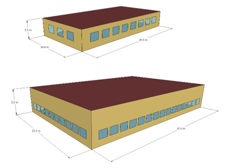
The first model was an office type building, 20 m by 10 m, having a 3 m height, and located at an intermediate floor. The longest facades were exposed to South and North and had 8 windows (1.5 m by 1.2 m) on each long side and 3 on each short side. U factor was 0.642 W/m2K for walls, and 2.735 W/m2K for windows. In the first occupation pattern the building was considered to be occupied by 20 persons, from 8 am to 8 pm, Monday to Friday. During this time a constant load of 2 kW was assumed for equipment, and 800 W max for lighting (dimmable as a function of natural lighting in order to keep a constant illuminance level of 100 lx at the center of the room). In the remaining time, a constant power of 25 W for lighting and 25 W for equipment were considered. In the second occupancy pattern, the building was considered to be occupied by 20 persons, from 8 am to 2 pm, and by 10 persons from 2 pm to 8 pm, Monday to Friday, and by 10 persons from 8 pm to 2 pm during weekends. Equipment and lighting loads were varied proportionally according to the occupation rate. In all the cases ventilation was assumed as 0.1 volumes per hour, during the occupancy hours, the heating system was assumed to be turned on November 15th to March 31st, with a setpoint temperature of 20°C, and a setback temperature of 16°C. From June 15th to September 15th the cooling was turned on with a setpoint temperature of 26 °C and a setback temperature of 30°C.
The second model was an industrial type building, 30 m by 20 m, having a 5 m height. The longest facades were exposed to South and North and had 15 windows (1.5 m by 1.2 m) on each side. U factor was 0.934 W/m2K for walls, 0.615 W/m2K for the ceiling, and 2.735 W/m2K for windows. In the first occupancy pattern the building was supposed to be occupied by 50 persons, from 8 am to 8 pm, and by 25 persons in the rest of the day, with no variation during weekends. Ventilation was assumed as 0.3 volumes per hour. During this time a constant load of 8 kW was assumed for equipment during the day, and halved during the night. For lighting the power was 2.5 kW during the day (dimmable as a function of natural lighting in order to keep a constant illuminance level of 150 lx at the center of the room) and 1.25 kW during the night. In the second occupancy pattern the building was supposed to be occupied by 15 persons during the whole day, with no variation during weekends. Ventilation was assumed as 0.1 volumes per hour. A constant load of 2 kW was assumed for equipment, while for lighting the power was 2.5 kW during the day (dimmable as a function of natural lighting in order to keep a constant illuminance level of 150 lx at the center of the room) and 1.25 kW during the night. The heating system was turned on November 15th till March 31st, with a setpoint temperature of 18°C. From June 15th to September 15th the cooling was turned on with a setpoint temperature of 26 °C.
All the simulations to collect the time series to be analyzed were carried out using EnergyPlys v. 8.9 software. In order to determine the heating and cooling energy consumptions in a simple and straightforward way, and also avoid making assumptions on more detailed plant characteristics, an “IdealLoadAirSystem” with no outdoor air was considered. This EnergyPlus object returns both the heating and cooling energy required to meet the temperature set-points that have been provided. Such loads were then converted into electric energy by conventionally assuming that a HVAC system with a COP equal to three (both for heating and cooling) provided them.
Among the different output variables that can be returned by the software, hourly values of those more likely to be monitored by the smart pole were considered. Thus, outdoor air temperature, relative humidity, wind speed, and global horizontal illuminance levels were used. With reference to the indoor environment, only indoor air temperature and carbon dioxide (CO2) concentration were collected, together with energy consumptions taken as a whole and subdivided as a function of the typology.
With reference to the weather conditions, all the analyses were carried out using the climate data for Bari/Palese Macchie. Data were taken from the IWEC2 (International Weather for Energy Calculations) database developed by ASHRAE within the Research Project RP-1477, “Development of 3012 Typical Year Weather Files for International Locations” [17], and from the Italian IGDG dataset. In this way, two years were available in order to better test the predictive accuracy of the models.
Figure 1. 3D models of the analyzed spaces representing an office and an industrial building
2.2 Machine learning methods
The ANN was implemented using the neural network toolbox in Matlab [18]. To learn the parameters of the ANN (i.e. the weights between neurons and biases) the network training was carried out by means of a Bayesian regularization algorithm. A two-layer feed-forward network with sigmoid hidden neurons and linear output neurons was used. The estimation of the number of neurons in each layer is one of the most difficult tasks, which is generally carried out using a trial and error procedure. In this case, 10 neurons were used as a starting point, but they were subsequently reduced to 8, after some testing. Daily values of partial and total energy consumption were used as target values. Hourly values were not considered at this stage as the fluctuations were too large, and, considering the availability of only outdoor parameters, it seemed preferable to focus only on daily data. Similarly, daily averages of the outdoor temperature, relative humidity, wind speed, total horizontal illuminance (beam+diffuse) were calculated and used as input parameters, together with the day of the week, the day of the year, and the possibility to have the heating and cooling system turned on or not. The latter parameters proved very important in order to correctly estimate aggregate (total) energy consumptions.
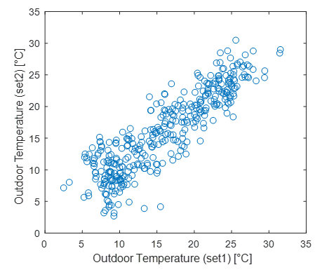
In a first “static” test, the ANN was trained by taking into account the results obtained using one of the two reference years, and subdividing the sample into three parts, randomly extracted, corresponding to 70% for the training, 15 % for the validation, and 15 % for the testing. To estimate the ANN performance, traditional metrics like root mean square error (RMSE) and regression coefficient R were used. However, with reference to the specific case, an extended testing was performed by taking into account a whole second year of simulations (obtained using the second weather file), and by measuring the RMSE in this second case. As shown in Figure 2, the mean outdoor temperatures referred to the same day may differ quite significantly, thus providing a good reference of the reliability of the predictive accuracy of the ANN. Finally, all the performance calculations were made both with and without indoor temperature as input parameter, to better understand the importance of this additional information.
As anticipated, the same analysis was carried out, at least in exploratory form, also by means of a NARX model, while keeping the same basic settings in terms of training set and method (Bayesian regularization). The delay in the network (the number of samples taken into account to predict each value) was set to 3, and the number of neurons was kept at 8, as it proved also for ANN to be a good choice.
Once the preliminary investigation was carried out, so that the best set of input parameters was selected, a final “incremental” test was designed in order to simulate actual working conditions of the predictive network. In fact, under real world conditions the amount of data to be used for training is going to increase continuously, with the ANN dynamically re-training as soon as new data are available. So, in order to broaden the time horizon, a third year was added to the simulation by repeating the EnergyPlus calculations using a different weather file, relative to the closest station, namely that of the city of Brindisi, 120 km south of Bari. At this point, in order to limit the calculation burden, the ANN was re-trained every week, gradually increasing the input dataset, and testing its performance on the subsequent week. RMSE was calculated every time in order to understand also the training time after which the ANN starts providing reliable results.
Figure 2. Scatterplot of the mean daily outdoor temperatures resulting from the two datasets referred to the city of Bari used to train and test the ANN
3.1 Office building
3.1.1 Occupancy pattern #1
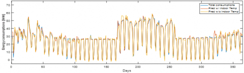
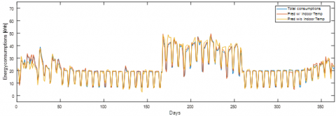
The office building is characterized by a markedly periodical behavior. Results of the training and testing sets demonstrated the good accuracy that the ANN is able to provide in predicting daily consumptions. Weekly cycles were well respected, and peaks and sudden fluctuations due to outdoor conditions found a good match in predicted values. In quantitative terms, during the testing on the first year RMSE on daily consumptions was 1.8 kWh and 1.5 kWh, respectively for the input set with and without indoor temperature. However, when the whole second year was considered (Figure 3), RMSE increased to 1.9 kWh for the input data with indoor temperature, and to 2.7 kWh for the set without it. The largest errors appeared in the reduced input dataset during the cooling season, while both datasets had a few problems at the beginning of the heating season in autumn. The analysis with the NARX method (Figure 4), yielded a significantly worse performance, with RMSE raising to about 4.4 kWh when applied to the “second” test year, independent of the input data set used.
3.1.2 Occupancy pattern #2
When the 2nd occupancy pattern was used, results were better than those obtained with the first one. In quantitative terms, during the testing on the first year RMSE was 1.0 kWh and 1.2 kWh, respectively for the input set with and without indoor temperature. However, when the second year was considered (Figure 5), RMSE increased to 1.1 kWh for the input data with indoor temperature, and to 2.5 kWh for the set without it. The agreement was very good, with the largest variations taking place during the cooling season. Again. the use of the NARX method provided significantly worse performance with errors between 4.1 and 4.9 kWh, depending on the input dataset.
Figure 3. Plot of simulated and predicted values of daily consumptions for office building (1st occupancy pattern) during 2nd year
Figure 4. Plot of simulated and predicted values of daily consumptions for office building with NARX method during the 2nd year
Figure 5. Plot of simulated and predicted values of daily consumptions for office building (2nd occupancy pattern) during 2nd year
3.2 Industrial building
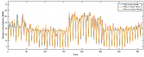
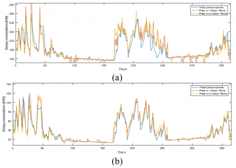
The industrial building offered a completely different pattern of energy use, showing no variation between weekdays and weekends in terms of equipment, thus providing a constant term which somewhat stabilized fluctuations particularly during intermediate seasons (Figure 6). Given the volume of the space and the high ventilation rate, significant heating and, particularly, cooling loads, were observed despite the reduced setpoint temperature in winter. Cooling loads, were clearly influenced by the internal gains due to equipment and lighting.
During the testing on the first year RMSE for daily consumptions was 6.0 kWh and 3.9 kWh, respectively for the input set with and without indoor temperature. However, when the second year was considered, RMSE increased to 17.1 kWh for the input data with indoor temperature, and to 15.5 kWh for the set without it (Figure 6a). The largest errors clearly appeared during the cooling season, with the ANN overestimating target data by 40% if the constant equipment load was included, but the relative variation skyrocketed if the equipment term was not included. So, in order to better understand the nature of the problem, in the subsequent analyses the equipment load was not included in the energy demand (which is actually more realistic as in an industrial site it will likely have a separate metering system). A detailed comparison between simulated and predicted values showed some odd behaviors like those appearing around day 240. Among input data, only wind speed was unusually high during those days, so training was repeated after excluding that parameter from the dataset. The test over the second year yielded a RMSE of 10.0 kWh when using indoor temperature and of 12.4 kWh when it was excluded.
A further improvement was obtained by including in the input dataset the energy consumption of the previous day, which yielded a RMSE equal to 7.8 kWh and 8.2 kWh, respectively with and without indoor temperature. A few significant inaccuracies remained between day 40 and day 50, when outdoor temperatures were at a minimum. Attempts to replace illuminance with radiation per area (assuming that a more expensive sensor might be used on the smart pole), only returned a small improvement with RMSE dropping to 6.5 kWh, but errors still appeared in the same days.
Even in this case, use of NARX method did not yield any improvement but, conversely, returned a significantly worsened performance with RMSE raising to 12.4 kWh and to 16.6 respectively when indoor temperature was included or not in the input dataset.
3.2.2 Occupancy pattern #2
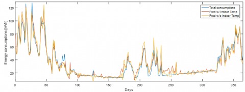
The second occupancy pattern was characterized by significantly lower equipment loads (and, hence, internal gains). Thus, this time heating loads largely prevailed over cooling loads. Use of the standard set of input parameters showed the same limitations already observed in the first occupancy pattern. In fact, RMSE was 12.6 kWh when using indoor temperature and 12.1 kWh when it was excluded. Replacement of wind speed with day-before energy consumptions caused, as already observed, a large improvement in prediction accuracy, as the RMSE dropped to 5.8 kWh when using indoor temperature, and to 6.8 kWh when it was excluded. Replacement of illuminance values with solar radiation rate per area barely affected the results, with no significant variation in RMSE values.
Application of the NARX method yielded a RMSE of 14.7 kWh and 13.8 kWh respectively with and without indoor temperature included among input data.
Figure 6. Plot of simulated and predicted values of daily consumptions in industrial building (1st occupancy pattern) using: a) ANN with original set of input data; b) ANN with modified input data, removing wind speed and including previous-day consumptions
Figure 7. Plot of simulated and predicted values of daily energy consumptions in industrial building (2nd occupancy pattern) using: ANN with modified set of input data, removing wind speed and including previous-day energy consumptions
3.3 Incremental-training analysis
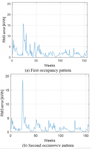
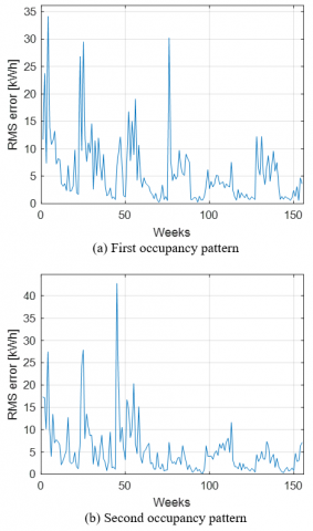
As anticipated, the final test was carried out by replicating the actual incremental behavior of the forecasting system, by means of weekly updates of the input data set. For this purpose, the input dataset was kept to a minimum by excluding wind speed and indoor temperature, while day-before consumptions were included as they proved to be important in the previous discussion. With reference to the office building, with the first occupancy pattern, the analysis showed (Figure 8a) that during the first year several inaccuracies occurred with RMSE calculated on a weekly basis, often higher that 5 kWh, resulting in very large relative errors. However, during the subsequent years the prediction performance was generally good, with only occasional problems, resulting in a RMSE of 1.8 kWh averaged over the third year (showing a substantial improvement when compared with the “static” value obtained under the same conditions for the 2nd year).
When the second occupancy pattern was considered, the same positive trend was observed (Figure 8b), with RMSE calculated on a weekly basis slowly decreasing, yielding even after the first nine months good results, with only occasional peaks exceeding 4 kWh. On a yearly basis, RMSE in the third year was 1.2 kWh, against a value of 1.8 kWh obtained in the second year. If compared with the RMSE resulting from the “static” test without indoor temperature (which was 2.5 kWh) a clear advantage appears.
The incremental training yielded even larger improvements when applied to the industrial building. In fact, with reference to the first occupancy pattern (Figure 9a), while the static analysis showed RMSE values around 8 kWh (with little variations depending on the indoor temperature inclusion in the dataset), the incremental training clearly showed its benefits reducing RMSE to 7.3 kWh during the second year, and to 4.5 kWh during the third, with weekly values showing larger, but steadily decreasing, fluctuations which kept exceeding the 5 kWh limit during the cooling season, but, given the higher absolute values of the target, resulted in smaller relative errors.
Finally, with reference to the second occupancy pattern, which was characterized by milder cooling consumptions and higher heating consumptions, the adaptive training also yielded several benefits (Figure 9b). In fact, the decreasing trend in RMSE calculated on a weekly basis was clearly visible, with values exceeding 5 kWh in a few occasions mostly during the winter season, resulting in a mean percent error of 8.6%. The yearly averaged RMSE was 5.6 kWh during the second year (the corresponding static value was 6.8 kWh), and it further dropped to 4.1 kWh during the third year.
Figure 8. Plot of weekly averaged RMS errors calculated during the adaptive training process with reference to office building under
Figure 9. Plot of weekly averaged RMS errors calculated during the adaptive training process with reference to office building under
The potential of machine learning techniques to predict energy consumption in office and industrial buildings was investigated in this paper. Target data were obtained by means of dynamic energy simulation for several buildings, using the EnergyPlus software. Among the different techniques, a two-layer feed-forward artificial neural network was investigated, together with another one using a non-linear autoregressive model with exogenous input. Among them, the first one showed clearly better performance in term of predictive accuracy, with a more stable behavior and considerably reduced day-by-day fluctuations.
In terms of input parameters, the analysis showed that the availability of indoor temperature typically improves the prediction accuracy when heating and cooling loads are involved. Among the outdoor parameters wind speed proved scarcely effective and was consequently removed from the final dataset. Conversely, previous-day energy consumption proved to be an essential input in order to improve accuracy, particularly for the industrial building where the magnitude of the heating and cooling loads was quite large and the availability of that additional parameter contributed to better adapt temperature variations to energy consumptions.
Finally, a simulation of the actual incremental training process was carried out, assuming that the ANN is re-trained every week. Results showed the best performance in all the cases, also using the input dataset without indoor temperature, with the performance of the network reaching acceptable levels after the first year, and significantly improving, nearly halving the RMS error, after the second one.
Further investigations are under way in order to investigate the potential of other prediction methods and, possibly, extend the ANN to also predict hourly values instead of daily values.
This paper was funded within the framework of the National Operative Program (PON). SE4I – Smart Energy Efficiency & Environment for Industry” (PON ARS01_01137).
[1] U.S. Energy Information Administration. Use of energy in the United States explained. https://www.eia.gov/energyexplained/
[2] Jamil M, Mittal S. (2017). Building energy management system: A review. 14th IEEE India Council International Conference, INDICON.
[3] Modoni GE, Veniero M, Trombetta A, Sacco M, Clemente S. (2017). Semantic based events signaling for AAL systems. Journal of Ambient Intelligence and Humanized Computing 9(5): 1311-1325. https://doi.org/10.1007/s12652-017-0534-0
[4] Mohamed N, Al-Jaroodi J, Jawhar I. (2018). Service-oriented big data analytics for improving buildings energy management in smart cities. 14th International Wireless Communications and Mobile Computing Conference, IWCMC 2018 8450469: 1243-1248. https://doi.org/10.1109/IWCMC.2018.8450469
[5] Al-Ali AR, Zualkernan IA, Rashid M, Gupta R, Alikarar M. (2017). A smart home energy management system using IoT and big data analytics approach. IEEE Transactions on Consumer Electronics 63(4): 426-434. https://doi.org/10.1109/TCE.2017.015014
[6] Modoni GE, Sacco M, Terkaj W. (2016). A telemetry-driven approach to simulate data-intensive manufacturing processes. In Proc. 49th CIRP-CMS. https://doi.org/10.1016/j.procir.2016.11.049
[7] Modoni GE, Trombetta A, Veniero M, Sacco M, Mourtzis D. (2019). An event-driven integrative framework enabling information notification among manufacturing resources. International Journal of Computer Integrated Manufacturing 32(3): 241-252. https://doi.org/10.1080/0951192X.2019.1571232
[8] Ahmad T, Chen H, Guo Y, Wang J. (2018). A comprehensive overview on the data driven and large scale based approaches for forecasting of building energy demand: A review. Energy and Buildings 165: 301-320. https://doi.org/10.1016/j.enbuild.2018.01.017
[9] Chapaloglou S, Nesiadis A, Iliadis AP, Antoniadis PI, Kakaras E. (2019). Smart energy management algorithm for load smoothing and peak shaving based on load forecasting of an island's power system. Applied Energy 627-642. https://doi.org/10.1016/j.apenergy.2019.01.102
[10] Moghaddas-Tafreshi SM, Mohseni S, Karami S, Kelly MES. (2019). Optimal energy management of a grid-connected multiple energy carrier micro-grid. Applied Thermal Engineering 152: 796-806. https://doi.org/10.1016/j.applthermaleng.2019.02.113
[11] Yu D, Brookson A, Fung AS, Raahemifar K, Mohammadi F. (2919). Transactive control of a residential community with solar photovoltaic and battery storage systems. IOP Conference Series: Earth and Environmental Science 238(1): 012051. https://doi.org/10.1088/1755-1315/238/1/012051
[12] Ahmad AS, Hassan MY, Abdullah MP, Rahman HA, Hussin F, Abdullah H. (2014). A review on applications of ANN and SVM for building electrical energy consumption forecasting. Renewable and Sustainable Energy Reviews 33: 102-109. https://doi.org/10.1016/j.rser.2014.01.069
[13] Edwards RE, New J, Parker LE. (2012). Predicting future hourly residential electrical consumption: A machine learning case study. Energy and Buildings 49: 591-603. https://doi.org/10.1016/j.enbuild.2012.03.010
[14] Ahmad T, Chen H. (2018). Short and medium-term forecasting of cooling and heating load demand in building environment with data-mining based approaches. Energy and Buildings 166: 460-476. https://doi.org/10.1016/j.enbuild.2018.01.066
[15] Ahmad T, Chen H. (2018). Potential of three variant machine-learning models for forecasting district level medium-term and long-term energy demand in smart grid environment. Energy 160: 1008-1020. https://doi.org/10.1016/j.energy.2018.07.084
[16] Martellotta F, Ayr U, Stefanizzi P, Sacchetti A, Riganti G. (2017). On the use of artificial neural networks to model household energy consumptions. Energy Procedia 126: 250-257. https://doi.org/10.1016/j.egypro.2017.08.149
[17] ASHRAE. (2012). International Weather for Energy Calculations (IWEC Weather Files) Version 2.0.
[18] MATLAB R.2016b, Neural Network Toolbox.