Tahar Brahimi*![]() | Atallah Benalia
| Atallah Benalia![]() | Iyad Ameur
| Iyad Ameur![]()
© 2025 The authors. This article is published by IIETA and is licensed under the CC BY 4.0 license (http://creativecommons.org/licenses/by/4.0/).
OPEN ACCESS
This study addresses the challenge of formation control for multiple non-holonomic unicycle mobile robots, a critical aspect of energy-efficient multi-agent robotic systems. A novel Generalized Proportional-Integral-Derivative (GPID) controller is proposed, grounded in Generalized Proportional Integral control theory, to ensure robust trajectory tracking and formation maintenance under uncertainties and disturbances. A dynamic model of unicycle robots is derived, and the GPID controller is designed to regulate cooperative formations. Stability is rigorously established using Lyapunov theory. Extensive MATLAB simulations demonstrate the controller’s superior performance, achieving enhanced stability, reduced tracking errors, and robust disturbance rejection compared to conventional PID controllers. Evaluated formation patterns confirm the approach’s adaptability in dynamic, energy-constrained environments. The results validate precise trajectory tracking and reliable formation control, underscoring the GPID controller’s potential in advancing robust and scalable strategies for cooperative robotics.
cooperative robotics, formation control, generalized PID controller, multi-agent systems, non-holonomic robots, trajectory tracking, Extended State Observer
The control and coordination of multiple mobile robots have become critical in advancing autonomous systems, with applications spanning industrial automation, military operations, surveillance, and search-and-rescue missions. Formation control, which involves maintaining a predefined geometric configuration while navigating dynamic environments, is essential for enabling collaborative robot behavior [1-3]. Effective formation control demands precise trajectory tracking, robustness to external disturbances, and adaptability to environmental changes. Among mobile robots, unicycle-type robots are widely studied due to their simple yet practical motion dynamics. However, their non-holonomic constraints, which restrict lateral motion, pose significant challenges for achieving accurate and stable formation control.
Prior work on formation control can be broadly categorized into three approaches: leader-follower, virtual structure, and behavior-based methods [4]. Leader-follower strategies, as explored by Consolini et al. [5], rely on a designated leader robot to guide the formation, but they often suffer from single-point failures [2]. Virtual structure approaches, such as those by Ren and Beard [1], treat the formation as a rigid body, offering stability but lacking flexibility in dynamic environments. Behavior-based methods, like those Balasubramanian and Ascoli [4], combine multiple control objectives but can lead to unpredictable interactions among robots; classical Proportional-Integral-Derivative (PID) controllers are commonly employed across these approaches due to their simplicity and effectiveness in single-robot systems [6, 7]. However, PID controllers struggle with the complexities of multi-robot formation control, exhibiting limitations such as poor disturbance rejection, slow convergence rates, and inadequate handling of inter-robot dynamics and environmental uncertainties. These shortcomings result in tracking errors and formation instability, particularly under varying conditions.
To this end, this research proposes a Generalized Proportional-Integral-Derivative (GPID) controller that integrates Generalized Proportional-Integral (GPI) principles [8, 9] to address these limitations. The GPID controller enhances disturbance rejection, improves trajectory tracking accuracy, and ensures stable formation control for multiple non-holonomic mobile robots. Building on recent advances in GPID and ESO-based control [10, 11], this study proposes a novel decentralized formulation tailored for real-time multi-robot formation tracking under bounded disturbances, Hence, this study investigates the research question: How can a GPID controller improve the formation control and trajectory tracking performance of multiple non-holonomic mobile robots compared to conventional PID-based approaches?
Compared to classical PID controllers, which rely on three gains (proportional, integral, and derivative), the proposed GPID controller introduces additional generalized integral and derivative terms based on the GPI framework. These added terms enhance the system’s ability to reject time-varying disturbances and improve transient response. Structurally, GPID incorporates extended internal states that offer more flexible shaping of system dynamics [10]. As a result, GPID outperforms PID in scenarios requiring high precision and robustness, such as formation control under inter-robot coupling and external perturbations.
Contributions of this work include:
These contributions aim to advance the field by providing a robust and adaptive control strategy for multi-robot systems, with potential applications in complex, real-world scenarios.
The remainder of this paper is organized as follows. Section 2 formulates the multi‐robot model and cost functions, detailing assumptions and problem setup. Section 3 presents the control strategy, theoretical analysis of convergence and optimality. Section 4 describes the stability of the proposed control method, Section 5 reports simulation results, comparing performance against baseline approaches. Finally, Section 6 concludes with a summary of findings and outlines directions for future research.
This section presents the dynamic model for a team of N non-holonomic mobile robots tasked with maintaining a predefined formation while tracking a reference trajectory in a 2D environment with static obstacles. The model accounts for the non-holonomic constraints of unicycle-type robots, integrates discrete-time kinematics, and defines the control objectives for the proposed Generalized Proportional-Integral-Derivative (GPID) controller, which enhances formation stability and trajectory tracking under disturbances.
2.1 System overview
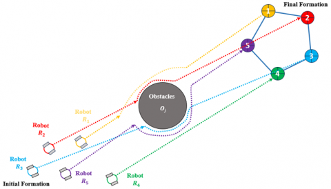
We consider a 2D workspace containing N unicycle-type mobile robots, each subject to non-holonomic constraints due to wheel rolling without slipping, and M static obstacles. The robots aim to maintain a specified geometric formation while tracking a reference trajectory defined by a virtual or physical leader [3]. The system objectives are threefold (see Figure 1):
Figure 1. Multi-robot coordination setup
Each robot is modeled as a circular agent with a fixed radius, operating under constrained unicycle dynamics, as described in. The environment includes static obstacles with fixed positions, and all positions are defined in a global Cartesian coordinate frame updated at discrete time steps $\Delta t$.
2.2 State variables
For each robot $i(i=1, \ldots, N)$, the state is defined by its position and orientation at time $t$:
2.3 Robot kinematics and dynamics
Each robot $i$ follows unicycle kinematics with non-holonomic constraints, restricting lateral motion [12] (i.e., no sliding perpendicular to the wheels). The kinematic model is given by:
$\begin{gathered}\dot{x}_i\left(t_n\right)=v_i(t) \cos \left(\theta_i\left(t_n\right)\right) \\ \dot{y}_i\left(t_n\right)=v_i(t) \sin \left(\theta_i\left(t_n\right)\right) \\ \dot{\theta}_i\left(t_n\right)=\omega_i(t)\end{gathered}$ (1)
where, $v_i(t)$ is the translational velocity and $\omega_i(t)$ is the angular velocity, both serving as control inputs. The nonholonomic constraint is expressed as:
$\dot{x}_{\imath}\left(t_n\right) \sin \left(\theta_i\left(t_n\right)-\dot{y}_{\imath}\left(t_n\right) \cos \left(\theta_i\left(t_n\right)\right)\right)=0$ (2)
Ensuring that motion occurs only along the robot's heading. the dynamic model, derived using the Lagrange formulation, accounts for the robot's mass $m_i$, moment of inertia $I_i$, and external forces/torques [13]. The dynamic equations are:
$m_i \ddot{p}_{\imath}=F_i(t), I_i \ddot{\theta}_{\imath}=\tau_i(t)$ (3)
where, $F_i(t)$ is the force and $\tau_i(t)$ is the torque, related to the control inputs $v_i(t)$ and $\omega_i(t)$ through actuator dynamics. For simplicity, we assume a direct mapping between control inputs and velocities, with disturbances modeled as additive terms $d_v(t)$ and $d_\omega(t)$ :
$v_i(t)=u_{v, i}(t)+d_v(t), \omega_i(t)=u_{\omega, i}(t)+d_\omega(t)$ (4)
where, $u_{v, i}(t)$ and $u_{\omega, i}(t)$ are the control signals generated by the GPID controller.
2.4 Control inputs
The control input vector for robot $i$ is:
$u_i(t)=\left[u_{v, i}(t), u_{\omega, i}(t)\right]^T$ (5)
where, $u_{v, i}(t)$ adjusts the translational velocity to track the reference trajectory and maintain formation, and $u_{\omega, i}(t)$ steers the robot to align its heading with the desired path. The GPID controller, incorporating Generalized Proportional-Integral (GPI) principles, computes these inputs to enhance disturbance rejection and tracking accuracy [14].
2.5 Cost function
Each robot $i$ optimizes a local cost function to balance the control objectives:
$\begin{gathered}J_i(t)=w_1 J_{c a, i}(t)+w_2 J_{f m, i}(t)+w_3 J_{t t, i}(t)+ w_4 J_{e e, i}(t)\end{gathered}$ (6)
where, $w_1, w_2, w_3, w_4$ are empirically tuned weights, and the terms are:
$\begin{gathered}J_{c a, i}(t)=\sum_{j \neq i} \exp \left(\frac{\left|p_i(t)-p_j(t)\right|^2}{\sigma^2}\right)+ \sum_{k=1}^M \exp \left(\frac{\left|p_i(t)-o_k\right|^2}{\sigma^2}\right)\end{gathered}$ (7)
penalizing proximity to other robots $\left(p_j(t)\right)$ and obstacles $\left(O_k\right)$, with $\sigma$ as the safety radius.
$J_{f m, i}(t)=\left|p_i(t)-\left(p_c(t)-d_i\right)\right|^2$ (8)
where, $d_i$ is the desired position of robot $i$ relative to the team centroid $p_c(t)$, ensuring adherence to the formation geometry.
$J_{t t, i}(t)=\left|p_i(t)-\left(p_r(t)-r_i\right)\right|^2$ (9)
where, $r_i$ is the desired offset from the reference trajectory $p_r(t)$, minimizing tracking error.
$J_{e e, i}(t)=\left|u_i(t)\right|^2$ (10)
penalizing excessive control effort to optimize energy consumption.
2.6 GPID controller design
The GPID controller extends the classical PID framework by incorporating GPI principles to handle non-holonomic constraints and external disturbances. For each robot $i$, the control inputs are computed as:
Linear Velocity Control (translation):
$\begin{gathered}u_{v, i}(t)=k_{p, v} e_{t t, i}(t)+k_{i, v} \int_0^t e_{t t, i}(\tau) d \tau+ k_{d, v} \dot{e}_{t t, i}(t)+u_{g p i, v}(t)\end{gathered}$ (11)
Angular Velocity Control (rotation):
$\begin{gathered}u_{\omega, i}(t)=k_{p, \omega} e_{f m, i}(t)+k_{i, \omega} \int_0^t e_{f m, i}(\tau) d \tau+ k_{d, \omega} \dot{e}_{f m, i}(t)+u_{g p i, \omega}(t)\end{gathered}$ (12)
where, $e_{t t, i}(t)=p_r(t)+r_i-p_i(t)$ is the tracking error, $e_{f m, i}(t)=p_c(t)+d_i-p_i(t)$ is the formation error, and $k_{p, . .}$, $k_{i, . .}, k_{d, . .}$ are proportional, integral, and derivative gains, respectively. The GPI term $u_{g p i, . .}(t)$ estimates and compensates for disturbances $d_v(t)$ and $d_\omega(t)$ using an Extended State Observer (ESO), enhancing robustness.
This dynamic model provides a foundation for the decentralized GPID control strategy, enabling precise formation control and trajectory tracking while mitigating the effects of non-holonomic constraints and environmental disturbances. The subsequent sections detail the control algorithm, stability analysis, and simulation results to validate the proposed approach.
This section presents the proposed Generalized Proportional-Integral-Derivative (GPID) control strategy for decentralized formation control of multiple non-holonomic mobile robots. We propose a hybrid strategy that integrates classical PID control with Generalized Proportional-Integral (GPI) principles to address the challenges of trajectory tracking, formation maintenance, and disturbance rejection in dynamic environments. The controller ensures robust performance under non-holonomic constraints and external disturbances by combining feedback control with disturbance estimation. The strategy is structured into modular components, detailed in the following subsections, and is validated through mathematical formulation and simulation results.
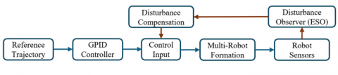
Figure 2. GPID control architecture for multi-robot formation
3.1 Overview of the GPID control framework
The GPID controller is designed to achieve three primary objectives: (1) precise tracking of a reference trajectory, (2) maintenance of a predefined formation geometry, and (3) robust collision avoidance with static obstacles and other robots [15, 16]. Unlike traditional PID controllers, which struggle with non-holonomic constraints and disturbances, the GPID incorporates a GPID module to estimate and compensate for external disturbances and model uncertainties. The controller ensures stable and accurate formation control by leveraging local state information and minimizing a multi-objective cost function, as defined in Section 2.5.
The control architecture is decentralized, with each robot $i (i=1, \ldots, N)$ computing its control inputs based on local measurements of its position $p_i(t)$ [17], orientation $\theta_i(t)$, and relative positions to the team centroid $p_c(t)$, reference trajectory $p_r(t)$, and obstacles $O_j$. Figure 2 illustrates the control framework, highlighting the interaction between feedback control, disturbance estimation, and control input computation.
3.2 Control laws
The GPID controller computes control inputs $u_i(t)= \left[u_{v, i}(t), u_{\omega, i}(t)\right]^T$, for each robot $i$, where $u_{v, i}(t)$ is the translational velocity input and $u_{\omega, i}(t)$ is the angular velocity input. These inputs are designed to minimize the cost function $J_i(t)$ defined in Section 2.5, which balances trajectory tracking, formation maintenance, collision avoidance, and energy efficiency. The control laws are:
$\begin{gathered}u_{v, i}(t)=k_{p, v} e_{t t, i}(t)+k_{i, v} \int_0^t e_{t t, i}(\tau) d \tau+ k_{d, v} \dot{e}_{t t, i}(t)+u_{g p i, v}(t)\end{gathered}$ (13)
$\begin{gathered}u_{\omega, i}(t)=k_{p, \omega} e_{f m, i}(t)+k_{i, \omega} \int_0^t e_{f m, i}(\tau) d \tau+ k_{d, \omega} \dot{e}_{f m, i}(t)+u_{g p i, \omega}(t)\end{gathered}$ (14)
where,
The controller ensures precise tracking by aligning the robot’s velocity with the reference trajectory while maintaining the desired formation geometry through angular adjustments. The GPID terms enhance robustness by compensating for external disturbances $d_v(t)$ and $d_\omega(t)$, as described in Section 2.3.
3.3 GPID module for disturbance rejection
The GPID module extends the classical PID framework by incorporating an ESO to estimate and compensate for disturbances and model uncertainties [18]. For each robot $i$, the ESO models the system dynamics as:
$\begin{aligned} \dot{v}_i(t) & =u_{v, i}(t)+d_v(t) \\ \dot{\omega}_i(t) & =u_{\omega, i}(t)+d_\omega(t)\end{aligned}$ (15)
where, $d_v(t)$ and $d_\omega(t)$ represent external disturbances (e.g., wind, uneven terrain) [19] and unmodeled dynamics. The ESO estimates the state variables ($v_i(t), \omega_i(t)$) and disturbances $\left(d_v(t), d_\omega(t)\right)$ using:
$\begin{gathered}\dot{\hat{v}}_i(t)=u_{v, i}(t)+\hat{d}_v(t)+l_{v, 1}\left(v_i(t)-\hat{v}_i(t)\right) \\ \dot{\hat{d}}_v(t)=l_{v, 2}\left(v_i(t)-\hat{v}_i(t)\right) \\ \dot{\omega}_i(t)=u_{\omega, i}(t)+\hat{d}_\omega(t)+l_{\omega, 1}\left(\omega_i(t)-\widehat{\omega}_i(t)\right) \\ \dot{\hat{d}}_\omega(t)=l_{\omega, 2}\left(\omega_i(t)-\widehat{\omega}_i(t)\right)\end{gathered}$ (16)
where, $l_{v, 1}, l_{v, 2}, l_{\omega, 1}, l_{\omega, 2}$ are observer gains, and $\hat{v}_i(t), \hat{d}_v(t)$, $\widehat{\omega}_i(t), \hat{d}_\omega(t)$ are the estimated states and disturbances. The GPID compensation terms are then computed as:
$u_{g p i, v}(t)=-\hat{d}_v(t), u_{g p i, \omega}(t)=-\hat{d}_\omega(t)$ (17)
The GPID module extends classical PID control by embedding integral and derivative actions with higher-order internal states, which shape the closed-loop dynamics more flexibly [20]. In the GPID framework, GPI generates feedforward-like terms that compensate for model uncertainties and nonlinearities. Physically, it acts as a dynamic corrector that adjusts control effort beyond instantaneous error, improving robustness and transient behavior. Its effectiveness is enhanced by the ESO, which estimates external disturbances in real time. The GPID term then cancels these disturbances by injecting an equal and opposite correction into the control signal, thus achieving active disturbance rejection.
The controller ensures robust performance by actively canceling estimated disturbances [21], improving tracking accuracy and formation stability compared to classical PID controllers, which lack such compensation.
3.4 Parameter selection and justification
The control parameters ($k_{p, v}, k_{i, v}, k_{d, v}, k_{p, \omega}, k_{i, \omega}, k_{d, \omega}$, $\left.l_{v, 1}, l_{v, 2}, l_{\omega, 1}, l_{\omega, 2}\right)$ are tuned to balance responsiveness, stability, and disturbance rejection [22]. The following guidelines justify the parameter choices:
These parameters are validated through simulations (Section 5), ensuring the controller achieves stable convergence and robust performance under varying conditions.
3.5 Collision avoidance mechanism
To ensure safe navigation, [15] the GPID controller incorporates a collision avoidance term in the cost function $J_{c a, i}(t)$ (Section 2.5). When the distance between robot $i$ and another robot or obstacle falls below a safety threshold $\sigma$, the exponential penalty increases sharply, prompting the controller to adjust $u_{v, i}(t)$ and $u_{\omega, i}(t)$ to steer away from potential collisions. The controller ensures collision-free navigation by prioritizing $J_{c a, i}(t)$ through a high weight $w_1$, as validated in simulations.
3.6 Implementation details
The GPID control algorithm is implemented in a decentralized manner, with each robot executing the following steps at each time step $\Delta t$:
The algorithm’s computational complexity scales linearly with N, as each robot processes only local information, making it suitable for large-scale multi-robot systems.
The proposed GPID controller is designed for decentralized execution, allowing each robot to compute its control input independently using only local measurements and communication with immediate neighbors. Each control cycle involves evaluating error vectors, computing control laws with fixed gain matrices, and estimating disturbances using a low-order ESO. These operations involve basic vector arithmetic and first-order filters, with constant time complexity per robot. As a result, the overall computational complexity scales linearly with the number of robots, making the controller suitable for real-time deployment in moderately large teams. Our MATLAB simulation achieves faster-than-real-time performance on standard hardware, and the structure lends itself to embedded implementation on resource-constrained microcontrollers, as also supported by related implementations in [10, 24].
This section analyzes the stability of the proposed Generalized Proportional-Integral-Derivative (GPID) control law for coordinating N non-holonomic mobile robots in formation while tracking a reference trajectory and avoiding collisions. The controller ensures asymptotic convergence to the desired formation and trajectory by leveraging Lyapunov stability theory. The analysis accounts for non-holonomic constraints, external disturbances, and the decentralized nature of the control strategy, with the GPID’s Generalized Proportional-Integral (GPI) module enhancing robustness. The following subsections define the Lyapunov function, derive stability conditions, and discuss robustness properties.
4.1 Lyapunov function
To assess stability [25], we define a Lyapunov candidate function $V(t)$ that quantifies the deviation of the multi-robot system from its objectives, to evaluate the system’s stability under the proposed GPID controller, we define the following error terms for each robot (i = 1, ..., N), let:
$\begin{gathered}e_{t t, i}(t)=p_r(t)+r_i-p_i(t) \\ e_{f m, i}(t)=p_c(t)+d_i-p_i(t) \\ e_{\theta, i}(t)=\theta_{d, i}(t)-\theta_i(t)\end{gathered}$ (18)
where, $\mathrm{p}_{\mathrm{r}}(t)$ is the reference trajectory, $\mathrm{r}_{\mathrm{i}}$ and $\mathrm{d}_{\mathrm{i}}$ denote the desired relative displacements for tracking and formation respectively, and $\theta_i(t)$ is the robot's heading.
We define the following Lyapunov candidate function for the overall system:
$\begin{gathered}V(t)=\sum_{i=1}^N\left[\frac{w_1}{2}\left|e_{t t, i}(t)\right|^2+\frac{w_2}{2}\left|e_{f m, i}(t)\right|^2+\right. \\ \frac{w_3}{2}\left(e_{\theta, i}(t)\right)^2+w_4 \int_0^t\left|e_{t t, i}(\tau)\right|^2 d \tau+ \\ w_5 \int_0^t\left|e_{f m, i}(\tau)\right|^2 d \tau\end{gathered}$ (19)
where, $w_1, w_2, w_3, w_4, w_5>0$ are cost function weights to balance trajectory tracking, formation cohesion, orientation accuracy, and energy use.
4.2 Stability analysis
We analyze stability by examining the time derivative of the Lyapunov function, $\dot{V}(t)$ [26], to ensure it is non-positive, indicating that the system converges to the desired state. Differentiating $V(t)$ yields:
$\begin{gathered}\dot{V}(t)=\sum_{i=1}^N\left[w_1 e_{t t, i}(t)^T \dot{e}_{t t, i}(t)+\right. \\ w_2 e_{f m, i}(t)^T \dot{e}_{f m, i}+w_3 e_{\theta, i}(t) \dot{e}_{\theta, i}(t)+ \\ \left.w_4\left|e_{t t, i}(\tau)\right|^2+w_5\left|e_{f m, i}(\tau)\right|^2\right]\end{gathered}$ (20)
Assuming that the ESO effectively estimates external disturbances and that orientation errors remain small, the error dynamics under the GPID controller yield negative contributions to $\dot{V}(t)$. In particular:
$\begin{gathered}\dot{V}(t) \leq-\sum_{i=1}^N\left[w_1 k_{p, v}\left\|e_{t t, i}(t)\right\|^2+\right. \left.w_2 k_{p, \omega}\left\|e_{f m, i}(t)\right\|^2+w_3 k_{p, \omega} e_{\theta, i}(t)^2\right]\end{gathered}$ (21)
The negative definite terms ensure $\dot{V}(t) \leq 0$, with equality only when $e_{t t, i}(t)=e_{f m, i}(t)=e_{\theta, i}(t)=0$. The integral terms in $V(t)$ and the GPI disturbance compensation prevent steady-state errors and ensure asymptotic convergence to the equilibrium state. By LaSalle's invariance principle, the system converges to the set where all errors are zero, implying stable formation and trajectory tracking.
4.3 Boundedness and robustness
The GPID controller ensures boundedness and robustness through the following properties:
The controller ensures robust stability by maintaining bounded tracking and formation errors even in the presence of disturbances, with the GPI module enhancing performance compared to classical PID controllers. The decentralized nature of the control law ensures scalability, as each robot computes its inputs independently, with computational complexity scaling linearly with N.
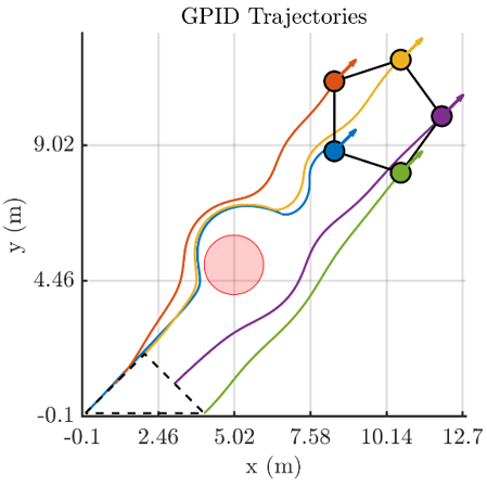
To assess the effectiveness of the proposed GPID controller in maintaining multi-robot formation and rejecting external disturbances, we simulate two control architectures: a classical PID and the GPID with disturbance estimation. Each robot begins in a triangular formation and is tasked with reaching a final pentagon formation while navigating around a circular obstacle. During the simulation, a disturbance force is injected selectively on GPID-controlled robots. This setup highlights the controller's robustness and its ability to preserve safe inter-robot distances while ensuring smooth convergence to the desired configuration.
(a) PID trajectories
(b) GPID trajectories
Figure 3. Comparison of PID and GPID trajectories
To ensure reliable formation control under uncertainty, each parameter in the proposed GPID architecture was carefully selected based on a combination of prior studies, theoretical guidelines, and task-specific tuning. For translational motion, the gains were initialized as $k_{p, v}=10, k_{i, v}=0.3$, and $k_{d, v}=$ 0.2 , selected to achieve fast convergence, eliminate steadystate error, and reduce overshoot respectively similar to the tuning strategies in [8, 10, 13]. Rotational control gains were set to $k_{p, \omega}=2.0, k_{i, \omega}=0.1$, and $k_{d, \omega}=0.3$, prioritizing heading stability and smooth reorientation [5, 12], the ESO bandwidth was selected $\omega_o=5.7$ to balance fast disturbance estimation with robustness, following guidance from ADRC literature [18, 19]. Obstacle avoidance used a repulsion gain $K_{\text {obs }}=3.0$, a decay factor $\alpha=1$, and a detection threshold $d_{\text {obs }}=7.0$ to ensure safe maneuvering near obstacles [15, 29]. The formation tolerance was set to $d_{\text {safe }}=0.07 \mathrm{~m}$, defining the maximum admissible deviation in inter-robot spacing [6, 13], cost function weights for local utility optimization were tuned to balance control priorities: $w_1=7$ (collision avoidance), $w_2=w_3=2$ (formation and tracking), and $w_4=0.2$ (control effort), based on common heuristics used in formation literature [2, 15, 30]. These values reflect the compromise between safety, accuracy, and energy efficiency. For robustness testing, a 0.2 N disturbance force was applied to GPID-controlled robots between 5 s and 10 s . The overall scenario involved transitioning from an initial triangular formation ([0,1,2,3,4]; [0,1,2,1,0]) to a regular pentagonal configuration centered at $(10,10)$ with radius 2 m . This geometric transformation, subject to obstacle interference, was selected to evaluate convergence, spacing preservation, and disturbance rejection in dynamic conditions, as recommended in formation benchmarks [1, 2, 5].
Figure 3 shows the comparison of multi-robot trajectories using (a) conventional PID and (b) GPID controllers. Both controllers guide five robots from an initial triangular formation (dashed lines) to a final pentagon formation (solid lines), while avoiding an obstacle (red circle). GPID demonstrates smoother paths with more consistent spacing and orientation, highlighting the benefit of active disturbance estimation and compensation through its integrated Extended State Observer (ESO). which actively estimates and cancels disturbances - a capability PID lacks. The ESO enables GPID to anticipate perturbations (as will be shown in the disturbance plot Figure 4), resulting in: 1) more precise trajectory tracking, 2) better maintained safety margins between robots, and 3) faster recovery after disturbances. While both controllers complete the formation task, GPID achieves superior performance with only marginally higher control effort, making it particularly valuable for real-world applications where environmental disturbances are common.
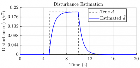
Figure 4. GPID disturbance estimation performance
The disturbance estimation results in Figure 4 demonstrate GPID's critical advantage over conventional PID control. The ESO accurately tracks the true disturbance profile (dashed line) within ≈2 seconds, enabling real-time compensation that PID cannot provide. This rapid convergence of the estimated disturbance explains GPID's superior performance in previous Figure 3 by actively canceling perturbations rather than just reacting to them, GPID maintains tighter formations and smoother trajectories. While PID must rely solely on error feedback, GPID's predictive capability prevents the overshoots and delays characteristic of PID's reactive approach. The plot clearly visualizes how GPID's disturbance-aware architecture achieves more robust control with only minimal additional computational cost.
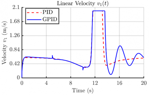
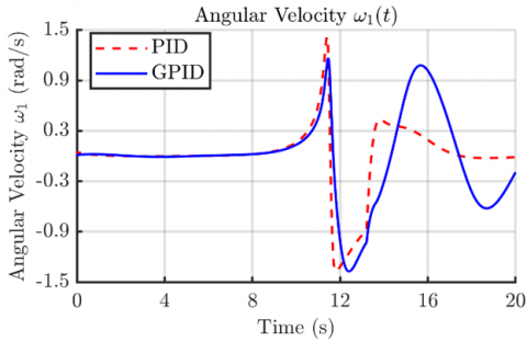
Figure 5 illustrates the control behavior of Robot 1 under both PID and GPID schemes during a disturbance event. In Figure 5a, GPID intelligently modulates the linear velocity, injecting an adaptive response that helps the robot maintain formation while remaining responsive to external forces. Figure 5b, shows that GPID produces smooth angular velocity adjustments, ensuring continuity in rotational motion even during sudden perturbations. A brief transient is observed in both profiles shortly after the disturbance onset, which is attributed to the Extended State Observer (ESO) rapidly estimating the disturbance. This short-lived oscillation reflects the dynamic learning process of the observer as it converges to the true force profile. Despite the initial mismatch, GPID quickly stabilizes and resumes nominal tracking demonstrating its ability to react decisively and maintain reliable control in uncertain conditions.
(a) Linear velocity $v_1(t)$
(b) Angular velocity $\omega_1(t)$
Figure 5. Comparison of linear and angular velocity profiles for PID and GPID
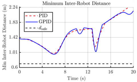
(a) Minimum inter-robot distance over time
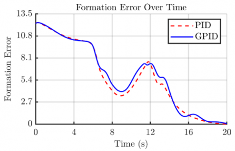
(b) Formation error with respect to the final shape
Figure 6. Formation-keeping performance comparison between PID and GPID
Despite being the only controller exposed to external disturbances, the GPID approach manages to maintain safe inter-robot distances and converge to the desired formation with impressive precision. As shown in Figure 6(a), the minimum distance between robots always remains above the safety threshold, reflecting the controller’s ability to preserve cohesion even under challenging conditions. Figure 6b further illustrates that GPID drives the robots to the final pentagon formation just as effectively as an undisturbed baseline, achieving near-zero error by the end. These results highlight GPID’s capacity to absorb unexpected changes while still delivering reliable, coordinated multi-robot behavior without compromising safety or formation quality.
This study presents a decentralized Generalized Proportional-Integral-Derivative (GPID) control framework for formation control of multiple non-holonomic mobile robots, addressing the challenges of precise trajectory tracking, formation maintenance, and collision avoidance in dynamic environments. By integrating Generalized Proportional-Integral (GPI) principles with classical PID control, the proposed approach enhances robustness against external disturbances and model uncertainties, overcoming the limitations of traditional PID controllers, such as poor disturbance rejection and slow convergence. The controller ensures stable and accurate formation control by leveraging an ESO to estimate and compensate for disturbances, as demonstrated through rigorous Lyapunov-based stability analysis.
The key contributions of this work include the development of a comprehensive dynamic model for non-holonomic unicycle robots, the design of a scalable GPID controller, and its validation through MATLAB-based simulations. The results confirm that the GPID controller achieves superior performance compared to conventional PID approaches, with improved tracking accuracy, faster formation recovery, and robust collision avoidance under varying conditions. The decentralized nature of the control law ensures linear scalability in computational complexity, making it suitable for large-scale multi-robot systems in applications such as industrial automation, surveillance, and search-and-rescue missions.
Future research will explore the integration of adaptive gain tuning to further enhance the controller’s adaptability to dynamic environments and heterogeneous robot teams. Additionally, the proposed GPID framework will be validated through real-world experiments using differential-drive mobile robots equipped with onboard sensors and embedded processors. These experiments will assess real-time performance under sensor noise, actuation limits, and communication delays. Hardware implementation will also investigate integration with ROS-based platforms and wireless multi-agent communication. This step will bridge the gap between simulation and field deployment, demonstrating the controller's viability in practical mission scenarios. This work thus advances the field of multi-robot systems by providing a robust, scalable, and theoretically grounded control strategy, paving the way for reliable autonomous coordination in complex, mission-critical environments.
This work has been supported by the LACoSERE Laboratory of University of Laghouat. The authors gratefully acknowledge the laboratory's technical assistance throughout the course of this research. This support has been instrumental in enabling the progress and development of the work presented here.
[1] Ren, W., Beard, R.W. (2020). Distributed Consensus in Multi-Vehicle Cooperative Control. Springer, London. https://doi.org/10.1007/978-1-84800-015-5
[2] Liu, Y., Liu, Z. (2023). Distributed adaptive formation control of multi-agent systems with measurement noises. Automatica, 150: 110857. https://doi.org/10.1016/j.automatica.2023.110857
[3] Azzabi, A., Nouri, K. (2021). Design of a robust tracking controller for a nonholonomic mobile robot based on sliding mode with adaptive gain. International Journal of Advanced Robotic Systems, 18(1). https://doi.org/10.1177/1729881420987082
[4] Balasubramanian, R., Ascoli, G. (2021). Behavior-based control for swarm robotics: A simulation study. International Journal of Heat and Technology, 39(5): 1345-1352. https://doi.org/10.18280/ijht.390506
[5] Consolini, L., Morbidi, F., Prattichizzo, D. (2021). Leader-follower formation control of non-holonomic robots with input constraints. Automatica, 125: 109432. https://doi.org/10.1016/j.automatica.2020.109432
[6] Chen, X., Jia, Y. (2020). Adaptive leader-follower formation control of non-holonomic mobile robots using active vision. IET Control Theory & Applications, 9(8): 1302-1311. https://doi.org/10.1049/iet-cta.2014.0019
[7] Liang, X., Wang, H., Liu, Y.H., Chen, W., Liu, T. (2020). Formation control of nonholonomic mobile robots without position and velocity measurements. IEEE Transactions on Robotics, 34(2): 434-446. https://doi.org/10.1109/TRO.2017.2776304
[8] Ma, Y., Zheng, G., Perruquetti, W., Qiu, Z. (2014). Motion planning for non-holonomic mobile robots using the i-pid controller and potential field. In 2014 IEEE/RSJ International Conference on Intelligent Robots and Systems, Chicago, IL, USA, pp. 3618-3623. https://doi.org/10.1109/IROS.2014.6943069
[9] Xiao, H., Li, Z., Chen, C.P. (2020). Formation control of leader-follower mobile robots’ systems using model predictive control based on neural-dynamic optimization. IEEE Transactions on Industrial Electronics, 63(9): 5752-5762. https://doi.org/10.1109/TIE.2016.2551740
[10] Eltayeb, A., Ahmed, G., Imran, I.H., Alyazidi, N.M., and Abubaker, A. (2024). Comparative analysis: Fractional PID vs. PID controllers for robotic arm using genetic algorithm optimization. Automation, 5(3): 230-245. https://doi.org/10.3390/automation5030014
[11] Cao, H., Li, Y., Liu, C., Zhao, S. (2023). Eso-based robust and high-precision tracking control for aerial manipulation. IEEE Transactions on Automation Science and Engineering, 21(2): 2139-2155. https://doi.org/10.1109/TASE.2023.3260874
[12] Nuño, E., Ortega, R., Basañez, L. (2022). Global consensus-based formation control of perturbed nonholonomic mobile robots with time-varying delays. Automatica, 141: 110294. https://doi.org/10.1016/j.automatica.2022.110294
[13] Saradagi, A., Muralidharan, V., Krishnan, V., Mahindrakar, A.D. (2020). Formation control and trajectory tracking of nonholonomic mobile robots. IEEE Transactions on Control Systems Technology, 28(6): 2250-2258. https://doi.org/10.1109/TCST.2017.2749563
[14] Wang, Z., Xu, T., Yang, K. (2023). Energy-efficient path planning for autonomous vehicles with obstacle avoidance. Robotics and Autonomous Systems, 162: 104366. https://doi.org/10.1016/j.robot.2023.104366
[15] Fallah, M.M.H., Janabi-Sharifi, F., Sajjadi, S. (2022). A visual predictive control framework for robust and constrained multi-agent formation control. Journal of Intelligent & Robotic Systems, 105(4): 72. https://doi.org/10.1007/s10846-022-01674-5
[16] Guo, B., Bacha, S., Alamir, M., Hably, A., Boudinet, C. (2021). Generalized integrator-extended state observer with applications to grid-connected converters in the presence of disturbances. IEEE Transactions on Control Systems Technology, 29(2): 744-755. https://doi.org/ 10.1109/TCST.2020.2981571
[17] Liu, T., Jiang, Z.P. (2020). Distributed formation control of nonholonomic mobile robots without global position measurements. Automatica, 115: 108883. https://doi.org/10.1016/j.automatica.2020.108883
[18] Han, J.Q. (2020). From PID to active disturbance rejection control. IEEE Transactions on Industrial Electronics, 56(3): 900-906. https://doi.org/10.1109/TIE.2008.2011621
[19] Ren, C., Li, X., Yang, X., Ma, S. (2020). Extended State Observer-based sliding mode control of an omnidirectional mobile robot with friction compensation. IEEE Transactions on Industrial Electronics, 66(12): 9480-9489. https://doi.org/10.1109/TIE.2019.2898586
[20] Fliess, M., Lévine, J., Martin, P., Rouchon, P. (1995). Flatness and defect of non-linear systems: Introductory theory and examples. International Journal of Control, 61(6): 1327-1361. https://doi.org/10.1080/00207179508921959
[21] Zheng, Q., Chen, Z., Gao, Z. (2020). A practical approach to disturbance decoupling control. Control Engineering Practice, 17(9): 1016-1025. https://doi.org/10.1016/j.conengprac.2009.04.005
[22] Vanchinathan, K., Valluvan, K.R., Gnanavel, C., Gokul, C. (2021). Design methodology and experimental verification of intelligent speed controllers for sensorless permanent magnet brushless DC motor. International Transactions on Electrical Energy Systems, 31(9): e12991. https://doi.org/10.1002/2050-7038.12991
[23] Lee, G., Chwa, D. (2018). Decentralized behavior-based formation control of multiple robots considering obstacle avoidance. Intelligent Service Robotics, 11(1): 127-138. https://doi.org/10.1007/s11370-017-0240-y
[24] Kowdiki, K.H., Barai, R.K., Bhattacharya, S. (2020). Autonomous leader-follower formation control of non-holonomic wheeled mobile robots by incremental path planning and sliding mode augmented tracking control. International Journal of Systems, Control and Communications, 10(3): 191-217. https://doi.org/10.1504/IJSCC.2019.100530
[25] Cajo, R., Guinaldo, M., Fabregas, E., Plaza, D. (2021). Distributed formation control for multiagent systems using a fractional-order proportional-integral structure. IEEE Transactions on Control Systems Technology, 29(5): 2234-2243. https://doi.org/ 10.1109/TCST.2021.3053541
[26] Pan, Z., Li, D., Yang, K., Deng, K. (2020). Multi-robot obstacle avoidance based on the improved artificial potential field and PID adaptive tracking control algorithm. Robotica, 37(11): 1883-1903. https://doi.org/ 10.1017/S026357471900033X
[27] Do, K.D. (2020). Nonlinear formation control of unicycle-type mobile robots. Robotics and Autonomous Systems, 127: 103468. https://doi.org/10.1016/j.robot.2006.09.001
[28] Abdulwahhab, O.W., Abbas, N.H. (2020). Design and stability analysis of a fractional order state feedback controller for trajectory tracking of a differential drive robot. International Journal of Control, Automation and Systems, 16(6): 2790-2800. https://doi.org/10.1007/s12555-017-0234-8
[29] Wang, L., Zou, Y., Meng, Z.Y. (2021). Stationary target localization and circumnavigation by a non-holonomic differentially driven mobile robot: Algorithms and experiments. International Journal of Robust and Nonlinear Control, 31(6): 2061-2081. https://doi.org/10.1002/rnc.5360
[30] Fierro, R., Lewis, F.L. (2020). Control of a nonholonomic mobile robot using neural networks. IEEE Transactions on Neural Networks, 9(4): 589-600. https://doi.org/10.1109/72.701174