Vijay Khare![]()
© 2023 IIETA. This article is published by IIETA and is licensed under the CC BY 4.0 license (http://creativecommons.org/licenses/by/4.0/).
OPEN ACCESS
This paper presents a novel method for optic disc (OD) detection in retinal images using a dictionary-based approach. The proposed method leverages the consistent properties of the OD region within retinal images, such as its circular shape, brightness, and blood vessel convergence at the center. In the training phase, a set of dictionary elements is composed using similar patterns selected from sub-images. The OD region can then be linearly represented in terms of these dictionary elements. The robustness of the detected OD center is ensured by verifying the presence of main blood vessel convergence at its neighborhood. The main blood vessels are obtained by estimating the background information using a large window sized median filter. To reduce the average computation time, OD detection is performed only on bright pixels in the test image, with pixel intensity assumed as the primary component for OD detection. These bright pixels are selected using local thresholding with a 15*15 block and Otsu algorithm. The proposed method is evaluated on three publicly available datasets, DRIVE, STARE, and DIARETDB1, comprising 210 retinal images. The experimental results show a success rate of 100%, 95.06%, and 98.8% for the three datasets, respectively.
fundus images, morphological operation, least angle regression (LARS), optic disc (OD), diabetic retinopathy (DR)
In recent days, it is observed that a major cause of visual deficiency is Diabetic retinopathy (DR) and Glaucoma. DR may be a dynamic retinal infection emerges due to diabetes, which can be maintained a strategic distance from or treated with lower fetched on the off chance that customary screening of a understanding enduring with diabetes is made by ophthalmologist. DR is recognized on the premise of pathologies (i.e., exudates, microaneurysm and hemorrhages) which can be effortlessly recognized in fundus pictures. These stores images captured employing a fundus camera which could be a computerized camera inserts magnifying lens at focal point conclusion. It gives tall quality pictures which permit the ophthalmologist to recognize the infection without affecting retina.
Concurring to Diabetes Atlas [1] larger part of 382 million individuals over the world enduring from diabetes are matured between 40 to 59 a long time. Whereas China, India and USA are best three nations with most extreme no of Diabetes quiet. To screen millions of individuals, expansive no of ophthalmologist is required. Hence, it is invaluable to create programmed DR location calculations to bolster the ophthalmologist. OD may be a brightest locale in retinal pictures and share comparable properties with exudates. Hence, for programmed location of DR it is obligatory to localize and expel OD pixels from retinal image [2-5].
Park et al. [6] proposed a template matching approach by considering 110*110 pixel sub-image with optic circle at the center from 25 color normalized retinal pictures and after that average them to create OD locale. This OD template image is matched with each pixel area in test retinal image and the point with maximum correlation is named as OD center. Mohanta et al. [7] proposed a calculation based on maximum intensity variation (since OD could be a shinning locale besides dark blood vessel). He used an 80*80 subregion over each pixel within the retinal image and searching for the locale with greatest escalated variety which is considered as optic nerve head. But it falls flat within the case of shinning exudates exist in retinal pictures since they lead to large variation in dark background.
A method based on convergence of blood vessel to the optic disc center using fuzzy technique is proposed [8]. But these algorithms are based on the accuracy of measurement of blood vessel. Otsu [9] proposed an algorithm based on properties of OD and identifying a brightest pixel using a repeated thresholding technique followed by obtaining the roundness of the object. Then OD is localized by using Hough transform. He verifies it on a DRIVE dataset of 40 retinal images. Another OD detection algorithm based on Hough transform and Morphological operation [10]. In which detects OD using Sobel operation for detecting edges and then circle is fit on these edge pixels using Hough transform. Both the algorithms are verified on 40 images from DRIVE dataset. Dehghani et al. [11] proposed a histogram matching approach for OD detection. He modifies the Osareh approach of template matching (12100 pixels) by matching histogram of red, green and blue channel individually to obtain the OD center. In literature, most of the algorithms use either the feature of OD or blood vessel convergence for OD detection. However, in proposed approach we use both OD feature and blood vessel convergence for OD detection. The article is organized as 'Anatomy of Retina' section, discussed the details of the retina. ‘Proposed Methodology’ section covers the detail of algorithm for OD localization followed by ‘Result and discussion'.
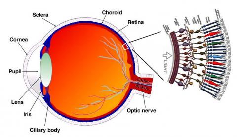
In study, it is observed that our eyes [12] resemble a camera where the light enters through the pupil and deflect on retina similar to camera film. The retina is an innermost light sensitive layer of tissues. It contains millions of photoreceptors absorb light signal and convert it to electrical signals transmitted to the brain. Figure 1 shows the side view of human eye.
Figure 1. Side view of the human eye [12]
Retina comprises of anatomical structures named as optic disc, blood vessels, macula and fovea. The first layer of the retina that receives light is called the nerve fiber layer. The majority of the retinal blood vessels are under this layer which nourishes the internal parts of the retina. While the outermost layer contains millions of photoreceptors which convert received light signal into electrical signals and deliver it through OD to the brain. These electrical impulses are transformed into images when they are received in the brain.
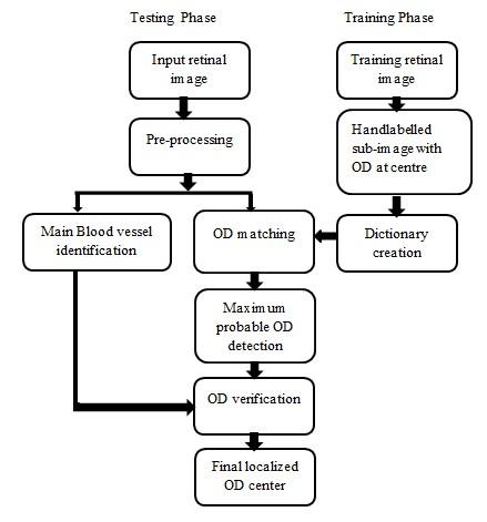
Most of the methods listed in literature performed well in normal retinal images. However, in the presence of exudates pathology their performance degrades. Block diagram of the proposed algorithm as shown in Figure 2 and summary of data set used shown in Table 1.
Figure 2. Block diagram of the proposed algorithm
3.1 Pre-processing
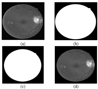
In pre-processing as shown in Figure 3 (a-d), we have performed two functions on the retinal images (i.e., resizing and boundary noise removal). Initially as image available in different datasets are of different size, we resize them to a standard size of 512*512 pixels. Secondly the image available in the datasets has a lighting effect on the boundary of the retina. To avoid the lighting effect on its boundary we find the binary mask of retinal image using the red channel of a test retinal image by thresholding it with a value of 20 percent of the maximum intensity since the pixel intensity outside the field of view (FOV) is nearly zero. After this we use Morphological erosion with disc shape of pixel diameter 15 to remove the unwanted boundary pixel by increasing the dark region as shown in Finally, logical ‘AND’ operation of resultant binary mask is performed with green channel retinal image.
Hubbard [13] observed that green and red channel of retinal image has more contrast i.e., spatial information then blue channel on the basis of broader histogram for red and green channel w.r.t blue channel. While blood vessels in the red channel behave as bright similar to background and in the green channel behave as dark in nature. Thus, we choose the green channel of retinal image for blood vessel identification. However, due to the presence of blood vessel in OD, its contour can be identified more accurately in the red channel. In this paper red channel is used for OD matching.
Figure 3. (a) Green channel of test retinal image with pathology; (b) mask obtained by thresholding; (c) mask with eliminated boundaries using morphological operation; (d) pre-processed green channel image obtained after and operation
3.2 Binary labelling
Binary labelling is an operation used to reduce the computation cost of the proposed algorithm. In this article it is assumed that OD is bright in nature, thus it is cost effective to search for OD only on bright pixel location [14, 15]. In binary labelling we obtain a binary image of green channel by thresholding it with threshold value 'T' such that all bright locations are selected. But due to non-uniform illumination and lightening effects 'T' cannot be a fixed value. The problem of selecting 'T' is solved using Otsu algorithm by selecting a local threshold in a block of size 15*15. Binary image obtained after thresholding is shown in Figure 4(c).
3.3 OD matching problem
The idea behind the OD matching is that feature of the optic disc (i.e., Circular shape, convergence of blood vessel, brightness) remains consistent and therefore subregion contain optic disc at center in all the images lie in a single subspace 'U' called as basis, and only the subregion from test image that contain optic disc at the center can be expressed as a linear combination of that subspace 'U'. While the other non OD region lies in different subspace 'V'.
3.4 Dictionary creation
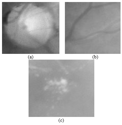
Initially 'm' retinal images for training purpose are selected. Now subregion of size n1*n2 pixels (i.e., 80*80) is selected from each image containing optic disc at the center to create the dictionary. The pixels of each sub region are arranged into column vector and then 'm' subregion selected above from training images are concatenated to form {U1, U2, U3... Um} named as Basis. A template with OD at center is shown in Figure 5 (a), while in Figure 5 (b) and Figure 5 (c) non OD template is shown. Since these non OD templates are not spanned in 'U' subspace, another subspace 'V' is included in the dictionary. 'V' is selected as a unity diagonal matrix with only one non-zero term in each column to represent each pixel value of the non OD template in a separate column. Thus, matrix 'V' is represented as {V1, V2, V3... Vn1*n2} sized [n1*n2, n1*n2] is an identity matrix and span the non OD templates. Hence dictionary is:
$\mathrm{A}=\left\{\mathrm{U}_1, \mathrm{U}_2, \mathrm{U}_3 \ldots \mathrm{U}_{\mathrm{m}}, \mathrm{V}_1, \mathrm{~V}_2, \mathrm{~V}_3, \ldots \mathrm{V}_{\mathrm{n} 1^* \mathrm{n} 2}\right\}$
$O r$
$\left[\left|\begin{array}{llllllllll}t_1^1 & t_1^2 & \ldots . & t_1^m &1&0&0&0&\ldots .\ldots .&0\\ t_2^1 & t_2^2 & \ldots . & t_2^m &0&1&0&0&\ldots .\ldots .&0\\ t_3^1 & t_3^2 & \ldots . & t_3^m &0&0&1&0&\ldots .\ldots .&0\\ \cdot & & \\ t_n^1 & t_n^2 & \ldots . & t_n^m&0&0&0&0&\ldots .\ldots .&1\end{array}\right|\right]$ (1)
where, tij indicates ith intensity pixel in jth sub-region with OD at center, n is equal to n1*n2 and m is no of training template with OD at center (m is selected as 20) [16, 17].
After the dictionary creation for OD detection, we choose templates of size [n1*n2] from the test image across the binary labelled pixel. It is converted into a column vector named as ‘Y’. Ideally, if given test subregion contain optic disc at its center it belongs to the subspace spanned by the basis {U1, U2, U3 ... Um} and coefficient vector would be {α1, α2, α3...αm, 0, 0, … 0}. While for subregion with no OD at the center represent in terms {V1, V2, V3 ... Vn1*n2} with coefficient vector would be {0, 0...0, β1, β2, β3 ... βn1*n2}.
Thus, any given sub image can be written as:
$\begin{aligned} & \mathrm{Y}=\alpha_1 * \mathrm{U}_1+\alpha_2 * \mathrm{U}_2+\alpha_3 * \mathrm{U}_3+\ldots \\ & +\mathrm{A}_{\mathrm{m}} * \mathrm{U}_{\mathrm{m}}+\beta_1 * \mathrm{~V}_1+\beta_2 * \mathrm{~V}_2+\beta_3 * \mathrm{~V}_3 \\ & +\ldots \ldots \beta_{\mathrm{n} 1^* \mathrm{n} 2} * \mathrm{~V}_{\mathrm{n} 1} * \mathrm{n} 2 \\ & O r \\ & \mathrm{Y}=\mathrm{A} * \mathrm{X}\end{aligned}$ (2)
where, X= [α1, α2, α3... αm, β1, β2, β3... βn1*n2] is a coefficient vector and A is dictionary matrix.
Figure 4. (a) Retinal fundus image; (b) processed green channel image of retinal image; (c) binary image obtained after thresholding in step2; (d) main blood vessel obtained from retinal image; (e) resultant image
Figure 5. Retinal image for red channel templates: (a) optic disc region; (b) blood vessel; (c) exudates
So, our problem of OD detection is changed into coefficient vector ‘X’ determination, where X is not a unique solution. The solution of X is optimal if,
$\mathrm{X}_0=\arg \min \|\mathrm{X}\|_0$ such that $\mathrm{Y}=\mathrm{A}^* \mathrm{X}$ (3)
where, $\|\cdot\|_0$ denotes l0 norm defined as non zero values in X. But this problem is NP-hard (i.e., there is no generalized procedure to solve it). Since it is assumed, template can be represented in terms of fewer vectors in dictionary 'A' thus it is similar to l1 least square regression problem and can be solved as least angle regression problem [18-20].
Table 1. Summary of retinal dataset used
|
Dataset |
Total no. of images |
Pathology images |
Size |
Field of view (FOV) |
|
DRIVE |
40 |
7 |
584*565 |
45° |
|
DIARETDB1 [21] |
89 |
84 |
1500*1152 |
50° |
|
STARE [20] |
81 |
50 |
605*700 |
35° |
Algorithm 1: To obtain ‘X’ coefficient vector.
1. Initialize all the coefficient values in X as zero.
$\hat{\mathrm{X}}$= {0, 0, 0, … 0};
2. Find the column vector (let Ai) in dictionary A, such that it is closer to Y. Set ith coefficient of X as unity, while making other coefficient zeros.
$\hat{\mathrm{X}}$= {0, 0, 0, …. 1, …. 0};
Thus predicted Y, $\hat{\mathrm{Y}}=\mathrm{A} \hat{\mathrm{X}}$.
1. Choose another vector (Aj) in dictionary A, next closest to the difference of Y and $\hat{\mathrm{Y}}$ . Then, coefficient vector $\hat{\mathrm{X}}$ = {0, 0, 0, … 1, … 0, 1, … 0};
2. Repeat step 3, Until squared error is minimized.
$\|\mathrm{Y}-\hat{\mathrm{Y}}\|_2 \leq \varepsilon$ (4)
where, ε is an error or tunning parameter. If ε is selected as a larger value than most of the coefficient tends towards zero, and if ε is selected as very small then it increases the computational cost. (ε = 01 is used in this paper).
$C_K=\frac{\sum_{i=1}^m \alpha_i}{\sqrt{\sum_{j=1}^n\left(1+\beta_j^2\right)}}$ (5)
And Ck is maximum, when the sum of α’s term is maximum and β’s term is minimum or 0 (i.e., when OD is at the center of sub-image).
3.5 Blood vessel analysis
Blood vessels are anatomical features of the retina which can be obtained as foreground information which can be detected as difference of image and background information. Background information in an image can be estimated using a filter of large dimension so that smaller blood vessel and noise information can be neglected. In this paper median filter of larger dimension (i.e., 30*30 to 70*70 pixels) is used to identify blood vessels. The prominent results are obtained at the median filter sized 50*50 pixels.
$\mathrm{I}_{\text {resultant }}=\mathrm{I}_{\text {median }}-\mathrm{I}_{\text {green }}$ (6)
where, Imedian is median filtered green channel image and Igreen is original green channel image.
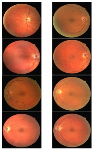
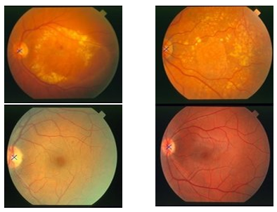
In Figures 6 and 7, the results of proposed method on DRIVE and STARE datasets are shown. In STARE datasets there is presence of large no of exudates pathology and we have detected OD with significant accuracy.
Figure 6. Optic disc detected in retinal images from DRIVE dataset
Now the threshold operation is applied on Iresultant to obtain the binary component of foreground information. The sequence of morphological erosion and dilation is performed on binary image to remove noise or minor blood vessel using structural elements of size (4 or 6). The resultant binary image after the morphological operation is shown in Figure 4 (d) [22-24].
3.6 Non OD image
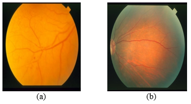
In some cases, while capturing retinal fundus images it may happen that an image is incorrectly captured as shown in Figure 8 (a) (from STARE dataset) and it does not contain Optic disc. To eliminate such images an option of reinserts the retinal image or incorrect retinal image is provided.
Figure 7. Optic disc detected in retinal images from STARE dataset
Algorithm 2: OD algorithm summary
To illustrate the performance of proposed algorithm we use three different datasets comprising of 210 retinal images with non-uniform illumination, different field of view and size.
The algorithm proposed in this paper is implemented in Matlab2013a, initially 20 images are randomly selected from three datasets for training purpose. In these 20 images OD center is manually marked and subimage of size 80*80 with OD at center is chosen. These subimages are downsampled to 20*20 and converted to column vector Since dictionary contains 20 training images it leads 'U' and 'V' is the identity matrix to deal every pixel noise. Thus, dictionary matrix 'A' has 400 rows, 420 columns. This dictionary matrix 'A' is remains unchanged for every test image and precomputed to reduce the computation time.
For test retinal image subimage of sized 80*80 is selected at the bright pixel location. It is downsampled to 20*20 and converted to column vector named as 'Y' of sized [400, 1]. After this linear regression equation Y=A*X is solved to compute the coefficient matrix ‘X’ leads to correlation matrix CK. The maximum correlated point named as OD center is verified by assuming a circular region of radius 15 pixels around it s.t. a logic '1' is assigned inside the circular region and logic '0' outside it. Then 'AND' operation is performed between circular region and binary image of the blood vessels. If no main blood vessel point is detected near the point CK, then this maximum correlated pixel is neglected and the next correlated point is chosen from correlated matrix CK. The average distance between estimated OD center and manually detected OD center is approximately 10.6 pixels in DRIVE dataset. The result of this algorithm is discussed in Table 2 [25-27].
In template matching [9, 10] approach a template contains OD at center sized 110*110 pixels (12100 pixels) are used as feature vector and to be matched at each location in the test image. This method is highly computationally expensive and improved by Dehghani [11]. In Dehghani algorithm he used a similar template approach, but in place of using pixel intensity as feature vector histogram matching approach is utilized. He obtains the separate histogram of red, green and blue channel for template region comprising of 256*3 (i.e., 768 features) gray levels and compared at each pixel location to compute the OD location. In our method instead of matching features at each location in retinal image. Intially, we utilize the brightness of OD as primary component of OD detection and locate bright pixels by thresholding operation. After this in place of comparing the pixel intensity or gray level, we represent the test template in terms of dictionary basis vector and only coefficient vector 'X' is computed. While computing coefficient vector CK it is observed that most of the coefficient in the coefficient vector 'X' is zero and few (up to 20) coefficients exist. In Table 3 we have shown result of comparison between different algorithms.
In proposed algorithm an idea of reinsert the image to reduce the possibility of incorrect OD detection has been introduced. It is based on the absence of high intensity pixel with major blood vessel in neighborhood. It leads to an advantage of detecting an image in STARE dataset (im0324) as no OD image as shown in Figure 8 (a). In Figure 8 (b), the characteristic of OD (i.e., brightness and convergence of blood vessel) cannot be seen clearly, therefore proposed method fails to localize the OD center.
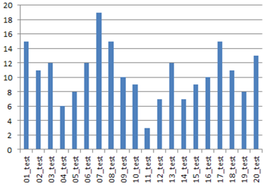
In Figure 9, the Euclidean distance between the estimated OD center and manually detected OD center obtained by the proposed method is shown. In proposed method we detect OD with an average tolerance of 10.6 pixels from the actual OD center, which is lesser than methods discussed in literature.
Table 2. Result of proposed algorithm in three datasets
|
Dataset |
Computational time (sec) |
Average distance (pixels) |
Minimum distance (pixels) |
Total no. of Images |
Correctly detected |
Success rate |
|
DRIVE [19] |
15 |
10.6 |
3 |
20 |
20 |
100 |
|
STARE [20] |
21 |
12.4 |
6 |
81 |
77 |
95.06 |
|
DIARETDB1 [21] |
19 |
14 |
5 |
89 |
88 |
98.08 |
Table 3. Comparison result of proposed algorithm on different datasets
|
Algorithm |
Success rate (%) |
Dataset |
Running time (sec) |
Average distance (in pixels) |
System configuration |
|
Rangayyan et al. [20] |
100 |
DRIVE |
2294 |
23.2 |
Intel core 2 Duo 2.5GHz 1.96Gb RAM |
|
69.1 |
STARE |
119 |
|||
|
Youssif et al. [21] |
100 |
DRIVE |
210 |
17 |
Intel core 2 Duo 2.5GHz 1.96Gb RAM |
|
98.77 |
STARE |
26 |
|||
|
Zhu et al. [10] |
90 |
DRIVE |
NA |
18 |
NA |
|
Osareh [22] |
58 |
DRIVE |
NA |
NA |
NA |
|
Sekhar et al. [14] |
85 |
DRIVE |
NA |
NA |
|
|
Mohanata et al. [7] |
100 |
DRIVE |
NA |
NA |
Intel core 2 Duo 2GHz 1.96Gb RAM |
|
64.1 |
STARE |
||||
|
Dehghani et al. [11] |
100 |
DRIVE |
27.6 |
15.9 |
Intel core 2 Duo 2.67GHz 3.24Gb RAM |
|
91.36 |
STARE |
11.4 |
|||
|
Park et al. [6] |
90.25 |
DRIVE |
4 |
NA |
NA |
|
Hoover and Goldbaum [8] |
89 |
STARE |
NA |
NA |
NA |
|
Our proposed |
100 |
DRIVE |
15 |
10.6 |
Intel Core i3 2.2GHz 2Gb RAM |
|
95.06 |
STARE |
21 |
12.4 |
||
|
98.08 |
DIARETDB1 |
19 |
14 |
Figure 8. Retinal images marked as no optic disc
Figure 9. Euclidean distance between the actual and detected center of the optic disc for DRIVE dataset
In this article a new method for localizing OD center is proposed and verified on three different datasets. The average distance between estimated and manually detected OD center is 23.2 and 119 pixels [6], 17 and 26 pixels [8] and 15.9 and 11.4 pixels [3] for DRIVE and STARE datasets respectively. While in proposed method average distance is 10.6, 12.4 and 14 pixels for the DRIVE, STARE and DIARETDB1 [25-27] datasets respectively. Therefore, OD center estimated in proposed method is more accurate as compared to algorithms [3, 6, 8]. In this article we have created a dictionary of OD template named as basis vector and predict the sub region in test image which can span these basis vector named as OD center. To further check the efficiency of our method we have implemented methods introduced [3, 9] on our system configuration. The average computation time obtained as 30sec [3], 6 min [9] and 15 seconds in our method for DRIVE dataset. The average computation time for our method on STARE dataset is more (i.e., 21 sec) due to presence of large size pathology as compared to DRIVE dataset. In this article to reduce the computation time we have performed OD detection only on bright pixels. It reduces the computation time, while our method failed for few unclear and blurred images. To avoid this obstacle in future we can capture or used a dataset with multiple images of a single patient and on the basis of contrast information highly contrasted image is chosen for OD detection.
[1] Aguirre, F., Brown, A., Cho, N.H., Dahlquist, G., Dodd, S., Dunning, T., Hirst, M., Hwang, C., Magliano, D., Patterson, C., Scott, C., Shaw, J., Soltesz, G., Usher-Smith, J., Whiting, D. (2013). IDF diabetes atlas: Sixth edition. International Diabetes Federation.
[2] Rathore, N.K., Pandey, D., Doewes, R.I., Bhatt, A. (2021). A novel security technique based on controlled pixel based encryption of image blocks for sharing a secret image. Wireless Personal Communications, 121(1): 191-207. https://doi.org/10.1007/s11277-021-08630-w
[3] Dhakad, N., Singh, R.K. (2020). Image enhancement techniques in medical domain: A survey. International Journal of Emerging Technology and Advanced Engineering, 9(10).
[4] Meshram, S., Kumar, S., Shukla, S. (2020). Enhanced robust and invisible of digital image using discrete cosine transform technique and binary shifting technique. International Journal of Emerging Technology and Advanced Engineering, 10(10): 113-118.
[5] Khan, R., Pillai, B. (2020). Enhanced digital image data hiding using image encrypted block histogram shifting method and Ardiem. International Journal of Emerging Technology and Advanced Engineering, 10(7): 41-46.
[6] Park, M., Jin, J.S., Luo, S.H. (2006). Locating the optic disc in retinal images. In International Conference on Computer Graphics, Imaging and Visualisation (CGIV'06), IEEE, 141-145. https://doi.org/10.1109/CGIV.2006.63
[7] Mohanta, J., Paramita, S., Singh, S.S. (2015). Detection of optical nerve head by using Gabor and mean filter. International Journal of Advanced Technology and Engineering Exploration, 2(2): 1-8.
[8] Hoover, A., Goldbaum, M. (2003). Locating the optic nerve in a retinal image using the fuzzy convergence of the blood vessels. In IEEE Transactions on Medical Imaging, 22(8): 951-958. https://doi.org/10.1109/TMI.2003.815900
[9] Otsu, N. (1979). A threshold selection method from gray-level histograms. In IEEE Transactions on Systems, Man, and Cybernetics, 9(1): 62-66. https://doi.org/10.1109/TSMC.1979.4310076
[10] Zhu, X.L., Rangayyan, R.M., Ells, A.L. (2010). Detection of the optic nerve head in fundus images of the retina using the Hough transform for circles. Journal of Digital Imaging, 23: 332-341. https://doi.org/10.1007/s10278-009-9189-5
[11] Dehghani, A., Moghaddam, H.A., Moin, M.S. (2012). Optic disc localization in retinal images using histogram matching. EURASIP Journal on Image and Video Processing, 1: 1-11. https://doi.org/10.1186/1687-5281-2012-19
[12] Kolb, H. (2011). Simple anatomy of the retina by Helga Kolb. Webvision: The Organization of the Retina and Visual System.
[13] Hubbard, L.D. (2009). Digital color fundus image quality: the impact of tonal resolution. The Journal of Ophthalmic Photography, 31: 15-20.
[14] Sekhar, S., Al-Nuaimy, W., Nandi, A.K. (2008). Automated localisation of optic disk and fovea in retinal fundus images. In 2008 16th European Signal Processing Conference, IEEE, 1-5.
[15] Ter Haar, F. (2005). Automatic localization of the optic disc in digital colour images of the human retina. Utrecht University, Institute of Information and Computing Sciences, Image Sciences Institute, 1-83.
[16] Akita, K., Kuga, H. (1982). A computer method of understanding ocular fundus images. Pattern Recognition, 15(6): 431-443. https://doi.org/10.1016/0031-3203(82)90022-X
[17] Sinthanayothin, C., Boyce, J.F., Cook, H.L., Williamson, T.H. (1999). Automated localisation of the optic disc, fovea, and retinal blood vessels from digital colour fundus images. British Journal of Ophthalmology, 83(8): 902-910. http://doi.org/10.1136/bjo.83.8.902
[18] Efron, B., Hastie, T., Johnstone, I., Tibshirani, R. (2004). Least angle regression. Ann. Statist, 32(2): 407-499. https://doi.org/10.1214/009053604000000067
[19] Gugulothu, V.K., Mohan Rao, S.K. (2020). Classification of IRS LISS-III images by using artificial neural networks. International Journal of Emerging Technology and Advanced Engineering, 10(4): 24-31.
[20] Rangayyan, R.M., Zhu, X.L., Ayres, F.J., Ells, A.L. (2010). Detection of the optic nerve head in fundus images of the retina with Gabor filters and phase portrait analysis. Journal of Digital Imaging, 23: 438-453. https://doi.org/10.1007/s10278-009-9261-1
[21] Youssif, A.A.H.A.R., Ghalwash, A.Z., Ghoneim, A.A.S.A.R. (2007). Optic disc detection from normalized digital fundus images by means of a vessels' direction matched filter. In IEEE Transactions on Medical Imaging, 27(1): 11-18. https://doi.org/10.1109/TMI.2007.900326
[22] Osareh, A. (2004). Automated identification of diabetic retinal exudates and the optic disc. Department of Computer Sciene, University of Bristol.
[23] Osareh, A., Mirmehdi, M., Thomas, B., Markham, R. (2002). Classification and localisation of diabetic-related eye disease. In European Conference on Computer Vision-ECCV 2002: 7th European Conference on Computer Vision, Springer Berlin Heidelberg, 502-516. https://doi.org/10.1007/3-540-47979-1_34
[24] Nahar, A., Sharma, S. (2020). Machine learning techniques for diabetes prediction: A review. International Journal of Emerging Technology and Advanced Engineering, 10(3): 28-34.
[25] Digital Retinal Images for Vessel Extraction (DRIVE).
[26] Structured Analysis of the Retina (STARE).
[27] DIARETDB1-standard diabetic retinopathy database calibration level. Accessed on 4 May 2023. https://www.kaggle.com/datasets/nguyenhung1903/diaretdb1-standard-diabetic-retinopathy-database